Browse our Frequently Asked Questions in relation to Depth Conversion & Velit VelPAK. If you have any queries, please do get in touch and contact us.
General
What software products does Equipoise Software develop?
Equipoise Software develops specialist geophysical software for depth conversion, velocity modelling, and seismic inversion. The main products include Velit (for the Petrel platform), VelPAK (for the Kingdom platform), Kingdom Seismic Inversion, and LogToVolume. These tools enable geoscientists to build accurate subsurface models, interpret seismic data, and quantify geological uncertainty for exploration and development projects. Velit VelPAK Kingdom Seismic Inversion LogToVolume.
Which geoscience platforms are compatible with Equipoise Software?
Equipoise Software tools integrate directly with the industry-standard interpretation platforms Petrel and Kingdom. Velit operates as a plug-in for Petrel, while VelPAK and the Seismic Inversion tools are available within the Kingdom environment. This allows geoscientists to incorporate advanced depth conversion and inversion workflows directly within their existing interpretation projects. Petrel Kingdom.
What types of velocity modelling methods are supported?
The depth conversion software includes a comprehensive library of industry-standard velocity modelling methods. These approaches can use both well velocity measurements and seismic processing velocities, allowing geoscientists to construct accurate velocity models even in areas with limited well control. The flexibility of these modelling approaches helps users tailor their workflows to the geological complexity of each project.
How do the software tools improve workflow efficiency for geoscientists?
Equipoise software uses guided Wizard-based workflows that help users step through complex modelling tasks in a structured way. This design approach reduces the learning curve for new users while also improving efficiency for experienced geoscientists performing advanced velocity modelling or inversion analyses.
What is meant by the “No Black Box” philosophy in Equipoise Software?
The software follows a “No Black Box” philosophy, meaning users can examine and adjust the modelling methods used in the workflow rather than relying on hidden algorithms. This transparency allows geoscientists to understand the assumptions behind their models, adapt workflows to their geological knowledge, and maintain full control over the interpretation process.
Depth Conversion and Uncertainty Concepts
What is depth uncertainty in seismic interpretation?
Depth uncertainty refers to the range of possible true depths that a geological horizon may lie at when converting seismic data from time to depth. Small variations in seismic velocity models, well calibration, or geological assumptions can lead to significant differences in predicted depth. Understanding this uncertainty is critical when planning wells, evaluating prospect volumes, or positioning geohazards. By quantifying uncertainty rather than relying on a single deterministic model, geoscientists can better assess exploration risk.
Why is it important to quantify depth uncertainty before drilling?
Even small depth errors can translate into large financial or operational risks when drilling a well. If a structure is deeper or shallower than expected, the well may miss the target reservoir or intersect hazards such as shallow gas. By quantifying uncertainty, geoscientists can evaluate a realistic range of outcomes and identify drilling locations with the lowest geophysical risk. Tools developed by Equipoise Software help quantify these uncertainties so that decisions are based on probability rather than a single assumed model.
What does “constrained stochastic multiple realisations” mean?
Constrained stochastic multiple realisations is a modelling approach that automatically generates many plausible versions of a depth model. Each realisation varies key inputs—such as velocity parameters—within geologically reasonable limits while honouring well and seismic data constraints. By analysing the ensemble of models, users can understand the likely distribution of structural depths and identify statistical outcomes such as P10, P50, and P90 cases.
How many stochastic realisations should typically be generated?
In many workflows, around 1,000 realisations are generated to capture a robust statistical representation of depth uncertainty. This large ensemble ensures that the full range of plausible geological outcomes is explored while still remaining computationally efficient. The resulting distribution of models can then be analysed to derive probabilistic depth surfaces and volumetric estimates.
How does constrained stochastic modelling differ from deterministic depth conversion?
Deterministic depth conversion produces a single “best estimate” depth map based on a chosen velocity model. While useful, it does not reveal how sensitive the result is to uncertainties in velocity, interpretation, or data quality. Constrained stochastic modelling, in contrast, generates many valid models around the best technical case, allowing geoscientists to quantify uncertainty and understand the full range of possible outcomes.
What are P10, P50 and P90 depth predictions?
These are statistical measures used to describe uncertainty in depth predictions.
P10 - A shallower case that only 10% of models exceed
P50 - The median or most likely depth estimate
P90 - A deeper case that 90% of models exceed
These probability-based depth estimates allow companies to evaluate structural risk and prospect volumes with a clearer understanding of uncertainty.
Can constrained stochastic modelling work with limited well control?
Yes. In many exploration settings, well data may be sparse or unevenly distributed. Modern depth conversion workflows combine available well velocities, seismic velocities, and geological constraints to build a best technical model. The stochastic realisations then explore the uncertainty around this model while still honouring the available data.
How does stochastic depth modelling help improve drilling decisions?
By understanding the range of possible structural outcomes, geoscientists can identify drilling locations that remain favourable across many possible scenarios. This reduces the risk of missing the target or encountering unexpected geological conditions. Quantified uncertainty also allows exploration teams to integrate geophysical risk directly into economic and volumetric evaluations.
Does stochastic modelling replace the need for a Best Technical Case model?
No. The Best Technical Case model remains the foundation of the workflow. It represents the geoscientist’s most realistic interpretation of the subsurface based on available data. Stochastic modelling then builds upon this model by exploring how uncertainties in the velocity field or interpretation could influence the resulting depth prediction.
How does depth uncertainty affect prospect volume estimates?
Structural depth uncertainty directly affects the estimated size of a reservoir or closure. If a structure is deeper or shallower than expected, the mapped closure area and hydrocarbon volume can change significantly. By analysing multiple stochastic realisations, geoscientists can derive probabilistic volume estimates and better understand the range of possible resource outcomes.
Velocity Modelling and Depth Conversion Workflows
Velocity Volume Generation - Can Velit create a 3d velocity cube from 2d stacking velocities?
This is a straightforward workflow for Velit. Simply import the stacking velocities for the 2d lines, generate a velocity model for that, and then design a pseudo-3d survey over the area of interest with 3 corner points, cell size and vertical increment. Velit can then populate this pseudo-3d with the 2d velocities which can then be exported to SEGY.
I can't perform Dix - is it because I have no layers in my model?
I have the 2D stacking velocities in Velit and I can display them but the options to perform Dix appears to have vanished. Is this because I don’t yet have any events/layers in my model?
Yes, you’ll need layers in the model; bung in dummy flat grid at max time e.g. 5 seconds to trick it.
How can I retrieve the V0 values at the wells in Velit?
You should be able to get a set of V0 values for your wells by doing the following method:
In the Optimise module:
![]() Select Edit Mode – Point
Select Edit Mode – Point
![]() From the Point Edit options that appear select User Edit
From the Point Edit options that appear select User Edit
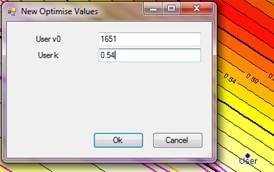
Click anywhere on the display. A User Point will be created and a box to edit the values for the User point will come up. Edit this to your V0 and K of the gradient of the curve you have:
Now in the XYZ tab of Optimise module set it as shown:
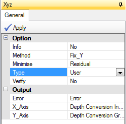
Note the Output X and Y will go into the named slots in the Model Tree for the Surface you are working with. Fixed Y has given fixed values of the K gradient, but the X values have gone into the Depth Conversion Intercept slot:
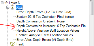
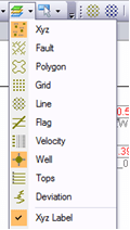
Click on this XYZ slot and turn XYZ and XYZ label on under Layers Visible in the Surface Module
How do I update my time grids in a VelPAK model? Will I have to set up the entire depth conversion again?
You should be able to get a set of V0 values for your wells by doing the following method:
In the Optimise module:
![]() Select Edit Mode – Point
Select Edit Mode – Point
![]() From the Point Edit options that appear select User Edit
From the Point Edit options that appear select User Edit
Click anywhere on the display. A User Point will be created and a box to edit the values for the User point will come up. Edit this to your V0 and K of the gradient of the curve you have:
Now in the XYZ tab of Optimise module set it as shown:
Note the Output X and Y will go into the named slots in the Model Tree for the Surface you are working with. Fixed Y has given fixed values of the K gradient, but the X values have gone into the Depth Conversion Intercept slot:
Click on this XYZ slot and turn XYZ and XYZ label on under Layers Visible in the Surface Module
How do I update my time grids in a VelPAK model? Will I have to set up the entire depth conversion again?
If the grids are simply updated (as opposed to introducing more grids into the model), it’s straightforward to import the new time grids into the model and re-do the depth conversion. All the parameters used by the depth conversion are stored in the model and won’t be lost when importing the revised grids, but there are some important caveats outlined below.
Before importing the new time grids, ensure they have the same cell size and extents as the grids used in the original VelPAK model. In VelPAK, click on a grid in the model tree and look at the ‘Properties’ table below to see this information. To get the new time grids into the VelPAK model, use ‘File > Open TKS…’, toggle on ‘Select Grids’, toggle off everything else and ensure that the ‘Data Import Mode’ is set to ‘Replace’. Work through the wizard as normal, ensuring the replacement grids go into the same layer numbers as the original grids.
What happens now depends very much on how the original depth conversion was made. If it was done via a workflow, simply load and re-run the workflow using the new time grids, and everything will automatically be updated (and the caveats below will be accounted for).
However, if the depth conversion was done ‘by hand’, if the grids have changed at any of the well locations, redo the layer definition in the ‘Layer’ module. Then any residual error correction in the model will have to be recomputed. This is easy enough, but takes several steps per layer in the model. For each layer:
Go to the Surface module Depth fly-out. The depth conversion parameters will be set there. Ensure that the ‘Input Error’ is set to zero, then press ‘Apply’ to depth convert without using the residual error correction
Re-compute the errors at the wells (Well module, Tie > Apply) – errors are stored in the XYZ Error slot
Re-generate the error grids from the XTZ error data (Surface > Grid)
Re-depth convert using the updated error grids (Surface > Depth & set ‘Input Error’ to the new error grid).
After each layer has been depth converted, save the model again, then transfer them back into the Kingdom project tree using ‘File > Save TKS…’.
These important caveats may or may not apply, depending upon how much and where the grids have changed:
If any of the depth conversion methods use ‘apparent’ interval velocities (e.g. “Interval Velocity vs. Depth to middle of Layer”), where top depths and grid times are used, if the grids have changed at the well locations then obviously the apparent interval velocities may have changed. In this case, go into the Curve module, open the ‘Generate’ fly-out, erase the current graph then press ‘Apply’ to regenerate the plot, before hitting ‘Surface > Depth > Apply’.
The above also applies if Optimisation was used; go to the Optimise module, open the ‘Generate’ fly-out and hit ‘Apply’ to re-run the optimisation before using ‘Surface > Depth > Apply’.
If stacking velocities have been used, changing the grids will change the interval velocities computed, so the interval velocity XYZ data will need to be regenerated & re-gridded.
If Profile data was generated from the time grids, these will need to be regenerated, as the horizons seen on the profile are separate from the grids.
How to depth convert using the “Salt Wedge Model 2” formula
Overview
The “Salt Wedge Model 2” function allows for depth conversion of a layer containing two mixed lithologies, a predominant layer and a subordinate layer (or layers) that may be variable in distribution. The layer is defined as usual by a top and a base grid, but is unusual in that an isochron grid (i.e. a time thickness map) containing the distribution of one of the lithologies is also provided as an input to the function.
Extra Inputs
- Isochron grid of one of the lithologies (matching the extents of the layer defining girds)
- Velocity of the predominant layer (grid or constant)
- Velocity of the mapped subordinate lithologies (grid or constant)
Example
A typical scenario is in the Zechstein formation in NW Europe. In the North Sea, this consists of fast velocity anhydrite rafts within a slower, more halitic layer.
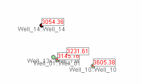
In this illustrative section, the anhydrite layers have been picked by top & base using 4 different interpretation horizons.
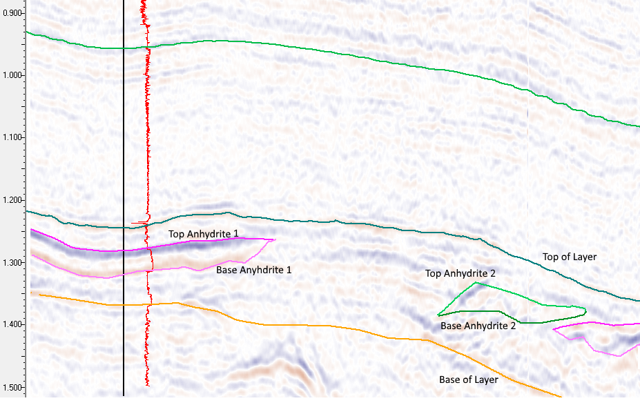
If there are multiple rafts stacked vertically, more horizons may be required.
The isochron of the anhydrite layer can be computed by subtracting the base from top anhydrite surfaces for each horizon pair, and then summing up & gridding. The isochron should be zero where no anhydrites exist, and the cumulative sum of the anhydrite time thickness layers vertically.
- Import this grid into the Velit model into a slot (I’ll assume General 01) for the appropriate layer.
- On the Surface display, open the pin-open the “Depth” fly-out, select the “Parameters” tab and set the “Formula” drop-down to “[General]SALT WEDGE MODEL 2” (& ensure “From” field is set to “User”).
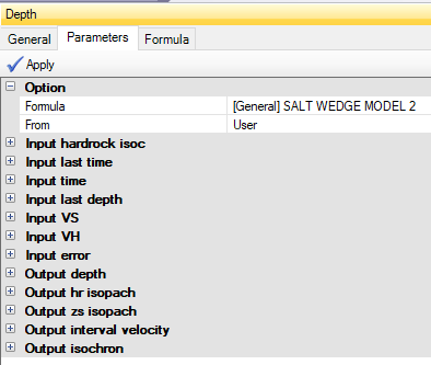
You can see the inputs are for “hardrock isoc”, the usual “last time”, “time”, “depth” and “error” slots, and the “VS” and “VH”. VS and VH are velocities for the primary & secondary lithologies respectively. In the Zechstein example, the slow velocity halites & faster anhydrites respectively.
Typically, the secondary (VH) velocity may be a constant (in this case I will use a very high 5900 m/s), but the VS velocity may be a constant or a grid. If you have good well coverage, you can deselect wells that don’t intersect with any of the secondary lithology and use the Wizard mapping function to map out the well velocities to create this grid.
- Copy the interval velocity grid to e.g. a General 02 slot, then turn the other wells back on as you may wish to perform residual error correction.
- Fill out the depth conversion dialog as follows (many of the parameters will be defaulted for you). Remember the first time you do a depth conversion, set the “Error” value to zero. The depth conversion computes the residuals which you can then grid and apply on a second depth conversion should you require.
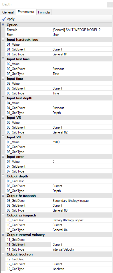
- Press the “Apply” button and the outputs will be computed. The isopachs for primary and secondary layers are put into the General 03 & 04 grids, but you can change these (but be careful not to overwrite your input isopach or velocity grids in General 01 & 02).
- If required, grid up the “XYZ > Error” values into an “Error” grid, then use this for the second conversion to tie the depth surface to the well markers.
Data Input and Integration
Importing ASCII Stacking Velocities Into VelPAK
ASCII stacking velocities cannot be converted to a SEG Y volume anywhere in Kingdom, or loaded into the main project database (unless converted to grids).
The stacking velocity ASCII file must conform to a simple, columnar format.
For 3d: Inline crossline time velocity
For 2d: Linename SP time velocity
where time is the time in MILISECONDS (not seconds!) and the velocity is in either metres/second or feet/second (matching the Kingdom project units).
Often files aren’t provided in this format, but they can be reformatted using the VelPAK ‘Tools > Scanit’ utility. The Scanit program has its own ‘Help’ menu which features some guided walkthroughs for using this tool. It can be tricky to get to grips with! If you have trouble using it, please forward your stacking velocity file onto the support team who can reformat it for you.
Before loading stacking velocities into a VelPAK model, be sure to load the survey(s) required into VelPAK by using ‘File > Open TKS…’ and turning on the ‘Select Surveys’ option.
For 3d surveys, VelPAK defaults to loading the co-ordinate information for every 10th inline. Inspect the stacking velocity file and see if it is decimated. To load all the velocities VelPAK must have loaded the corresponding trace coordinates from Kingdom (it won’t interpolate the cords).
For example, if the survey starts at 4154 but the stacking velocity file starts at 4160 and skips every 20th line, ensure you load the survey starting at 4160 with an increment of 20. If in doubt, load the entire survey by setting the inline increment to 1, it won’t affect performance significantly unless you are using the VelPAK ‘Profile’ mode.
Note that all trace coordinates are loaded for each inline, irrespective of the crossline selection, so you don’t need to explicitly load crosslines (unless you are dealing with complex profiles in the crossline direction).
Once co-ordinates are loaded, then proceed to load the stacking velocities using ‘File > Import > Profile Stack….’. Select the stacking velocity file, then for 3d surveys, ensure you set the ‘Prefix’ for the correct survey at the bottom of the dialog – it’s easy to miss.
For 2d lines, the survey name is in the imported file, but you do need to ensure the names in the file are an exact match for the names in Kingdom, or you will get an error message about coordinates not found.
Once the velocities are loaded, you can QC their position on the VelPAK ‘Surface’ map by using the ‘Layers Visible’ drop-down and toggling on ‘Velocity’. You should see pink blobs at the trace locations where stacking velocities occur (if there are blue ones, don’t worry about that, it just indicates they are located on the currently active line).
To QC velocity values, set the ‘Edit Mode’ drop-down to ‘Velocity’ then left-click on a pink blob to see a one-line summary in the ‘Console’ window, or use the middle-mouse button to see a pop-up of the values at that location.
To display the velocities in profile, open the ‘Velocity’ tab and you will see velocities for the current layer in the VelPAK model. If you click the ‘Surface’ tab (under the model tree) and set ‘Surface’ to 0, you should see all the velocities in the model plotted. Use the ‘Display’ fly-out and set ‘Well_overlay’ to ‘Yes’ to compare with well velocities.
Once the stacking velocities are loaded, there are numerous ways of incorporating them in the depth conversion. Popular techniques involve making a grid of interval velocities for each layer, calibrating stacking velocities to the well velocities and then depth converting, making pseudo-wells from stacking velocities and modelling functions from those, or kriging well velocities using the calibrated stacking velocities as an external drift function. It is impossible to recommend a particular method, as it will depend upon the data & distribution of the data in the project, the geology, geophysical constraints etc.
A good place to start with stacking velocities is the workflow system.
If you have no well velocity data, the simplest workflow is ‘Dix IntervalVelocity Multi.xml’ which does a direct conversion of the layer using interval velocities derived from stacking velocities using the Dix equation (see ‘Kingdom > Help > Tutorials > VelPAK > VelPAK Glossary’) for more information on the Dix parameter. On the ‘Velocity’ tab, apply the Dix scaling factor to your stacking velocities to compute the Dix interval velocities, then run the workflow.
Here is a screenshot of the full workflow for a 3 layer model that is depth converted using the Dix interval velocities directly:

If you have well data, and have performed Layer Definition and well calibration to prepare the well data, then it might be worth trying the ‘Dix Smooth and Calibrate.xml’ workflow, which scales the stacking interval velocities to the well interval velocities to give a more realistic result.
As the workflow runs, you can interact with the displays to ensure outlier well velocities are identified and removed from the scaling computation. If you do stop the workflow to deselect wells, ensure you re-run the workflow for that layer so the layer is depth converted before moving on to the next layer.
Importing Average Velocities into VelPAK/Velit
The standard GUI assumes the incoming velocity volume is an RMS (stacking) velocity volume.
Use the following procedure to import the data as an average velocities:
Import the average velocity volume as per usual as if it were RMS velocities; the import procedure creates an ASCII file on disk of inline/xline/time/RMSVelocity
Delete the velocities from the model (Edit > Delete Stacking Velocities > All Lines) then save the model (this is to ensure that if the Dix fly-out is used by mistake or in a workflow, the real average velocities aren’t overwritten).
Go to the model folder and locate the “import” subfolder
Edit stacking_velocity.dat using a text editor, and insert two columns of zeroes before the last column (so you have inline/xline/time/0/0/Velocity). The last column will be read by VelPAK/Velit as Average Velocity (the 5th column is read as depth). You can use ScanIt or a column editor such as “cream” if the file is too big for Excel.
In Velit/VelPAK, use “File > Import > Profile Stack…” and select the edited file; don’t forget to select the corresponding survey in the “Prefix” dropdown.
The velocities are imported as average; on the velocity display, you can plot the average velocities, convert them to XYZ data etc. as per usual.
Can you give me workflow of exporting the velocity volume that I created in VelPAK to import it in TKS to use it for dynamic depth conversion?
You can generate a velocity volume from your model using the “Velocity” tab, then the “Volume” fly-out.
First, select the survey using the “Survey” option; this will cause the survey extents to be filled in the remainder of the dialog. You can then manually adjust the Inline & Xline Min/Max values for the volume you wish to generate.
Time_Increment is the sample rate in milliseconds the volume will be generated at, and Time_Max is the time in milliseconds to generate the volume down to. Adjust these to match your seismic volumes in the Kingdom project.
Change Dimension to Average, as average velocity is the most convenient velocity volume for using in Kingdom, then set the filename in the File field. Press Apply to generate the volume as a SEG Y file. You can also use the Batch Execution (lightning flash) icon to generate the volume in batch, using multiple CPUs.
Once the volume generation is complete, there will be a SEG Y file in the “volume” folder of the model directory. You can import this into Kingdom as a seismic data type using “Surveys > Import SEGY Y…” in the usual fashion; use the default options for the SEG Y import, but ensure you store the volume as 16-bit or 32-bit, as 8-bit isn’t good enough to hold the dynamic range of velocities accurately.
Wells and Seismic Calibration
What are the preferred DT-log units: microsecs/m or microsecs/ft?
Velit always assumes that the sonic log is in microseconds/foot, even if the vertical units in the Kingdom project are metres. In the latter case, Velit will scale the log appropriately so that the displayed velocities are in metres/second.
Why don’t my Well Tops match up with my seismic event horizons on the Well Display?
You are using a sonic log – you need to calibrate the sonic log to a seismic event horizon.