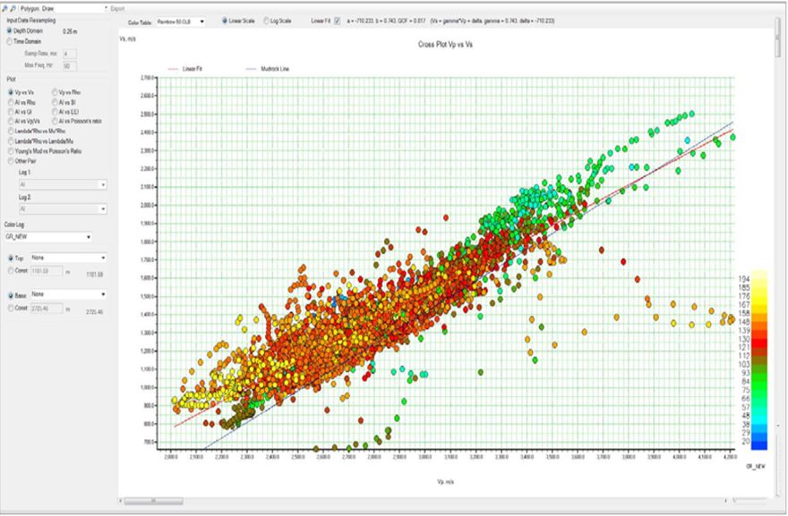
A detailed exploration of one of the key features from the Pre-Stack Inversion module in Kingdom’s Seismic Inversion suite. This module is driven by log input and includes a Cross-Plot feature, which allows users to select and display pairs of Elastic Parameters. While certain pairs are predefined, you have the flexibility to choose your own pairings—this includes combining petrophysical logs to discover correlations between elastic and petrophysical data.
Each point on the cross-plot represents a sample from the logs, and you can further enhance the visualization by selecting a third log to serve as a color bar, adding more detail to the plot. The data is automatically resampled to a depth resolution of 0.25 meters. For time domain cross-plots, the default sampling rate is adjustable between 1 and 20, with the maximum frequency range adjustable between 1 and 125 Hz.
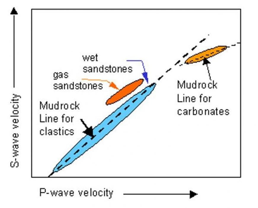
Polygons can be drawn on the cross-plot to isolate specific lithologies or fluid targets, such as gas sands, which can be clearly distinguished from background shale in an AI vs PR cross-plot.
The display supports both linear and logarithmic scales. When the linear fit is selected, the plot shows the linear regression along with values like the Goodness of Fit (GOF). Additionally, the plot will display the Mudrock line or Gardner’s Rule, depending on the selected parameter pairing—Vp vs Vs for the Mudrock line, and Vp vs Rhob for Gardner’s Rule.
- Mudrock Line: In rock physics and petrophysics, the Mudrock line (also known as Castagna’s equation) is an empirical relationship between P-wave velocity and S-wave velocity in brine-saturated siliciclastic rocks such as sandstones and shales.
- Gardner’s Rule: This rule connects seismic P-wave velocity with the bulk density of the lithology through which the wave passes. It helps infer lithology from interval velocities in seismic data. The constants used are typically calibrated using sonic and density well logs, but in the absence of this data, Gardner’s constants can serve as useful approximations.