Upon loading Kingdom Seismic Inversion, you are presented with an initial selection screen where you can select the type of Inversion you wish to perform. At this first step, you can select ‘Acoustic Impedance Inversion (and HiDef Vp)’ from the menu.
This option uses Simulated Annealing (SA) as the optimising technique and it enables you to perform a single-well operation, where you will typically want to target a window of 500 – 1000ms such that the wavelet is more appropriate for your area of interest. As part of the process, you can create an average wavelet from multiple wells in your survey area, if you want to encompass some spatial variation of your data. It is important to note however, that despite parameterising the Inversion from a well, the well isn’t used as part of the inversion itself, as the process involves a background starting model and the wavelet only.
Data Selection Screen
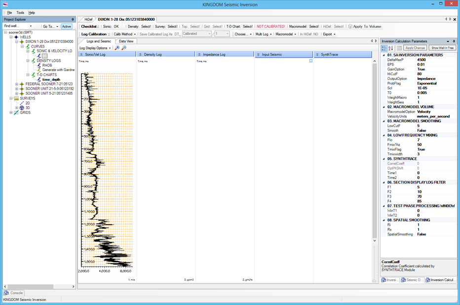
You’ll find a model tree to the left-hand-side of the main window and this process is much like Colored Inversion.
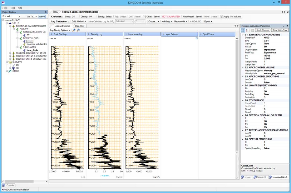
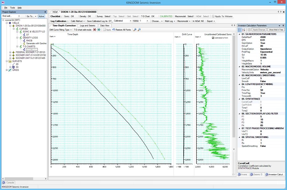
Firstly select your DT, under Curves > Sonic & Velocity Logs. Then select your Density Log and then your Time-Depth chart. You can see that the panel which runs along the top of the screen will change from ‘Select’ to ‘OK’ with each successive click for the respective data types.
Lastly you can select the amplitudes, with the software loading them and displaying the LogSeisMatch screen.
LogSeis Match Screen
A seismic trace near a well can be selected from a seismic data volume using a shortest distance criterion. However the trace selected in this way may not show a best match with the synthetic trace generated from the calibrated sonic log.
An alternative approach has been made so that a seismic trace is selected according to a match quality between seismic and log segments. All seismic traces within a defined neighbourhood of a well are compared to a segment of the log. The match is computed using their power and cross spectra.
The well is highlighted in black and the optimal seismic trace is highlighted as the red dot.
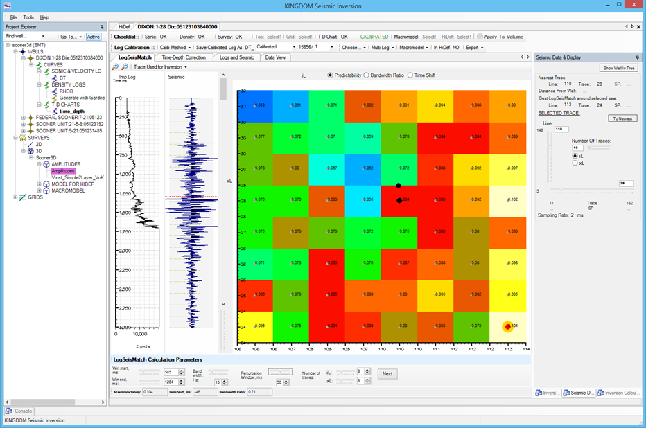
You proceed by selecting the window of interest. Here the selection is 1200ms and 1700ms for the start and end time respectively.
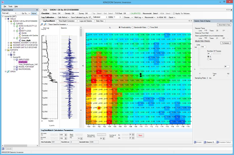
Next we can expand the search area around the well. In this example the In-Line and Cross-Line display has been adjusted from 8 to 20 traces around the well in each direction.
The blue colour denotes a low match predictability, and the yellow/white colour denotes a high match predictability.
In this example we can see that the optimal trace for using to match between the logs and the seismic is 8 traces away from the well (Optimal trace 102, well location trace 110). If we assume a 12.5m bin spacing for the data, the optimal trace in this dataset would be 100m away from the well. If this well were located on a fault boundary, it would not be appropriate to select a trace on the other side of the fault, and so you would choose the trace at the well location in preference.
The trace with a highest match quality is then selected and later used for well tie analysis, wavelet estimation and inversion job parameterisation. In addition, time shift errors between the log and seismic data can also be calculated and displayed for further assessing the quality of well ties.
We proceed by pressing the Next button which is flashing in green.
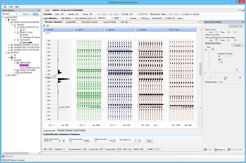
Wavelet Estimation Screen
A wavelet is a convolutional operator between log reflectivity traces and the seismic data. In this package, the wavelet is estimated by matching the log and corresponding seismic segments through the cross and power spectra of both segments (White, 1980).
The uncertainty of the estimation can be analysed by several factors such as predictability, smooth bandwidth ratio, correlation coefficient etc. The accuracy of the wavelet can be measured by the normalized mean square error (NMSE).
The wavelet estimation can be performed on each well, and their spectral characteristics are analysed. The package also allows external wavelets to be imported for inversion such as Hampton and Russell wavelet and other wavelets.
From Left to Right: The estimated wavelet; Log reflectivity; Real seismic trace; Synthetic seismic trace; Error trace. Predictability, bandwidth ratio and NMSE are also estimated.
On this screen a window start time of 1200ms and an end time of 1704ms has been selected. You are aiming to get a correlation coefficient of greater than 0.7, with a low Normalised Mean Square Error value.
We can look at the wavelet chosen by selecting the Wavelets and Spectra tab.
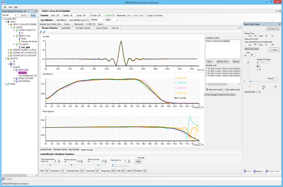
Wavelet Estimation – Wavelets & Spectra Tab
Top Left: Estimated wavelet
Top Right: Estimated wavelet of a fixed length
Bottom Left: Amplitude spectrum of the wavelet
Bottom Right: Phase spectrum of the wavelet.
If you want to import an external wavelet, you can select the Import Wavelet tab.

Wavelet Estimation – Import Wavelet Tab
On this screen you are able to select between importing a wavelet directly from The Kingdom Suite, the TKS option, from ASCII pairs as the EPS option, and from Hampson-Russell Suite, the HRS option.
When you are happy with your selected wavelet and the Correlation Coefficient and MNSE parameters, press the flashing green Next button to proceed. Alternatively, you may wish to create an average wavelet, using the wavelets derived from multiple wells across your survey area. To do this, select the Multiple Wavelets tab.

Wavelet Estimation – Multiple-Wavelets Tab
On this tab you can click on “Add from File” and select as many wavelets as you like from multiple wells in your dataset. Once all the wells have been imported, you can choose whether you want to align the wavelets with the positive peak, or the negative peak. The display will update dynamically depending on your selection, for QC purposes.
If you are happy to proceed with this option, you must tick the “Use Averaged Wavelet for SA Inversion” box and press the flashing green Next button to continue.
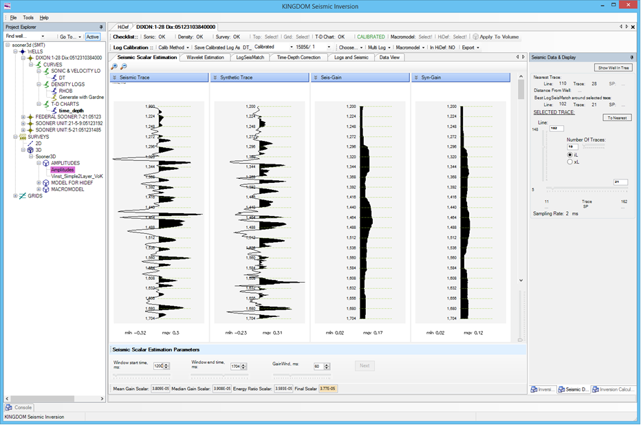
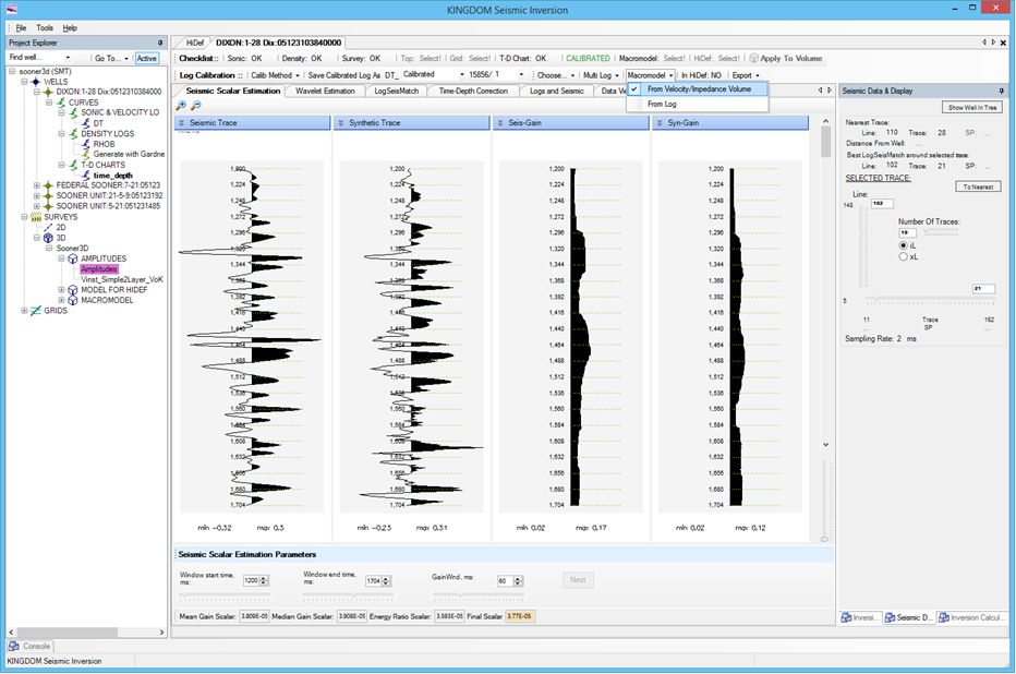
Seismic Scalar Estimation Screen
It is common that amplitudes of seismic data don’t match the amplitude range of a log reflectivity trace. In other words, when a derived wavelet is convolved with the log reflectivity, the resulting synthetic trace may have a different amplitude range from seismic data.
In order to properly calculate a misfit between synthetic and observed seismic data in the objective function computation, there is a need to estimate a scalar which can be applied to seismic data. In this package, the seismic scalar is automatically determined by comparing amplitude envelopes of synthetic and seismic traces. The scalar is then applied to seismic data before inversion begins.
From Left to Right:
Seismic trace
Synthetic trace
Amplitude envelope of seismic trace
Amplitude envelope of synthetic trace
A scalar is determined from the two envelopes and passed onto the parameter grid
You will see that the software is flashing ‘Select!’ at the top next to the Macromodel.
You proceed by selected your macromodel from either a Velocity/Impedance Volume, or from the well log.
It is worth reiterating that the macromodel used is only loosely coupled to the inversion, mainly as the starting point, and it does not use the log for the inversion at all.
Once you have selected the macromodel, press the flashing green Next button to continue.
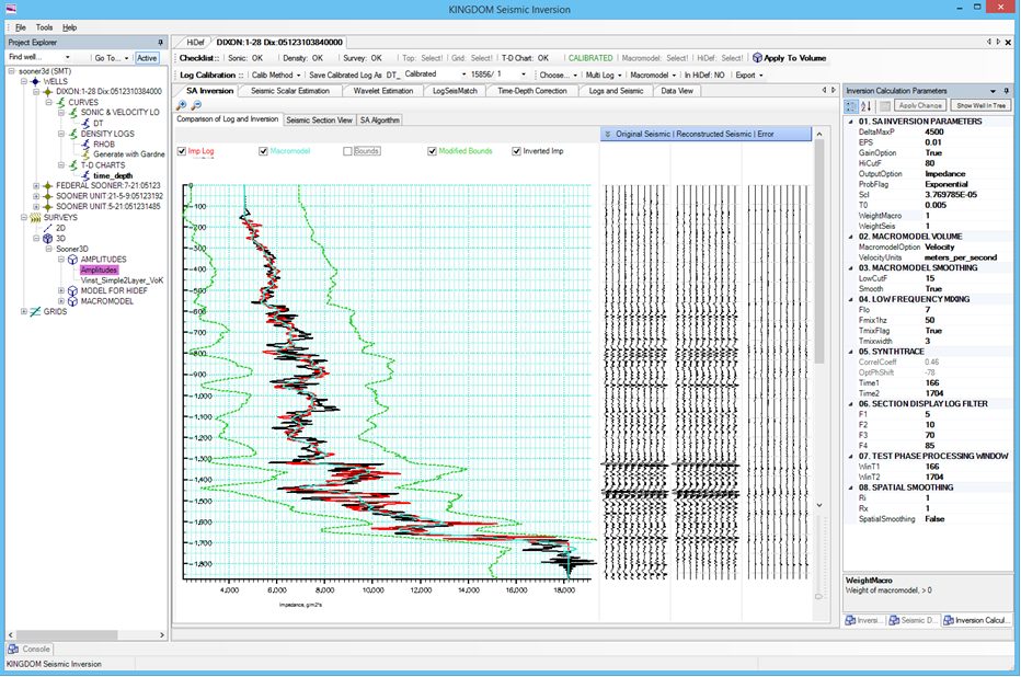
SA Inversion Screen
Once the wavelet and seismic scalar are estimated, the next step is to parameterise the inversion job. Parameters to be tuned include starting models, impedance perturbation windows, seismic scalar, seismic and macro-model weights, SA initial temperature, convergence tolerance etc.
Optimal job parameters are determined in such a way that the inverted impedance near the well shows a best match with impedance log and that the misfit between the synthetic trace and seismic trace is at its minimum.
The aim here is to visually minimise the error trace with your selection parameters.
You can also select to view the Seismic Section View or the SA Algorithm, by click on the respective tabs above the main graphical display.
When you are ready to proceed, press the Apply To Volume button at the top of the screen.
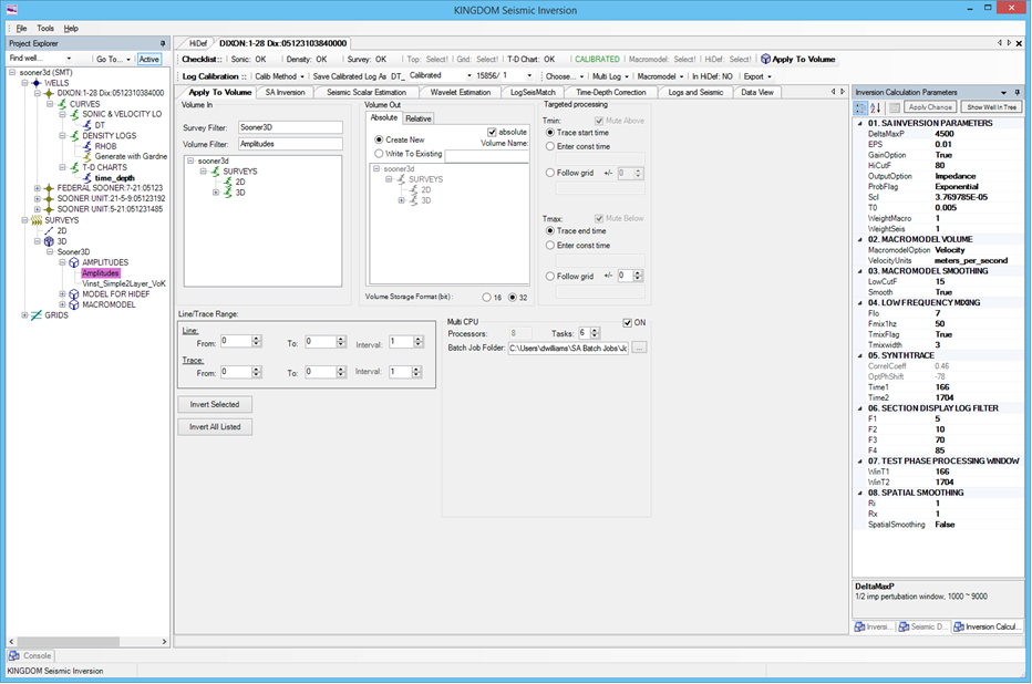
Apply To Volume Screen
SA volume inversion allows for the inversion of seismic reflectivity volumes using the wavelet and parameters optimally defined. Volumes or sub-volumes may be inverted, and processing windows using grids or constants specified.
Both absolute and relative inversion volumes may be generated.
SA volume inversion allows for the inversion of seismic reflectivity volumes using the wavelet and parameters optimally defined. Volumes or sub-volumes may be inverted, and processing windows using grids or constants specified.
You can also work with a Trace start and end time, to work from a Constant start and end time, or to Follow a Grid with a plus/minus selection around the grids of your choosing.
Simulated Annealing Inversion supports multi-CPU processing to increase throughput, whilst allowing the user to carry on working on other parts of the project. The typical processing time should be approximately 8 hours for a dataset of 40km x 60km using 8 cores in batch mode. It is worth noting that before running the whole job, you can create a subset volume of say 100 traces around the well on which you can test your parameters. This should take 30 minutes or so to process, such that in several hours, you could have 4 parameter selections to choose from, upon which you can use the optimal parameter selection for the whole job thereafter.
You can now see how easy SA Inversion is to run in Kingdom, with 4 screens to interact with and where you have full control over the parameters you wish to use to invert your seismic data.
There is presently a nuance that once the volume has completed its processing, that you need to shutdown Kingdom Seismic Inversion and Kingdom, then reopen Kingdom for the data to be visible in the software.
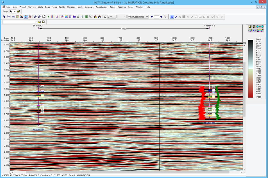
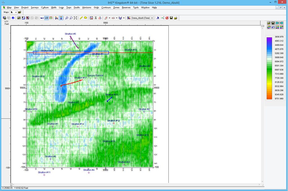
Kingdom Visualisation of Data
In this example, the first window shows the seismic data. You can see an anomaly in the middle of the dataset that is our main feature of interest. You can also note that the formation top markers in the log are shown within the bounds of the seismic (either at the peak or trough), rather than being at the zero crossing. This makes it potentially more challenging to perform your interpretation on.
By selecting the drop down we can now see the relative impedance volume generated by the SA Inversion.
It can be seen that the formation tops are now situated on the interface between the layers and that the anomaly in the central area of the screen is a low impedance body.

Here we can see the absolute acoustic impedance volume. It can been seen that the image is of higher resolution than the relative impedance volume, with the anomaly being better defined.

If we take a time slice through the anomaly we can see that it is a low impedance sand body.
If you would like to maximise the value of your seismic data and leverage additional attributes to improve its interpretability or if you’d like to know more about Kingdom Seismic Inversion then click here or to contact us for a free evaluation, e-mail us on sales@equipoisesoftware.com.
The software is provided by S&P Global (who we partner with for Kingdom) with perpetual and subscription pricing available on request. We offer a series of Teams meetings throughout the evaluation to help you quickly step up the learning curve and enable you to see the results for yourself.