This article covers the steps required to transfer data from Kingdom into VelPAK, and highlights several key points to ensure that your model will be built smoothly. Of great significance to this, it is vitally important to ensure that your data (sonic logs, formation tops, time grids, seismic velocities) have been thoroughly conditioned before you get to working in VelPAK. You can also note that the point at which Kingdom synchronises the ‘visible’ data with VelPAK is when you click on ‘Save Current Project’. As another point of good house keeping, it can be valuable to create a new author called VelPAK and populate that author with only the relevant data you want to use for the VelPAK model. Also, it can be useful to rename your Time Grids and Formation Tops to have 001, 002, 003, etc. in front, such that when you build the model, it is easy to get the layering right.
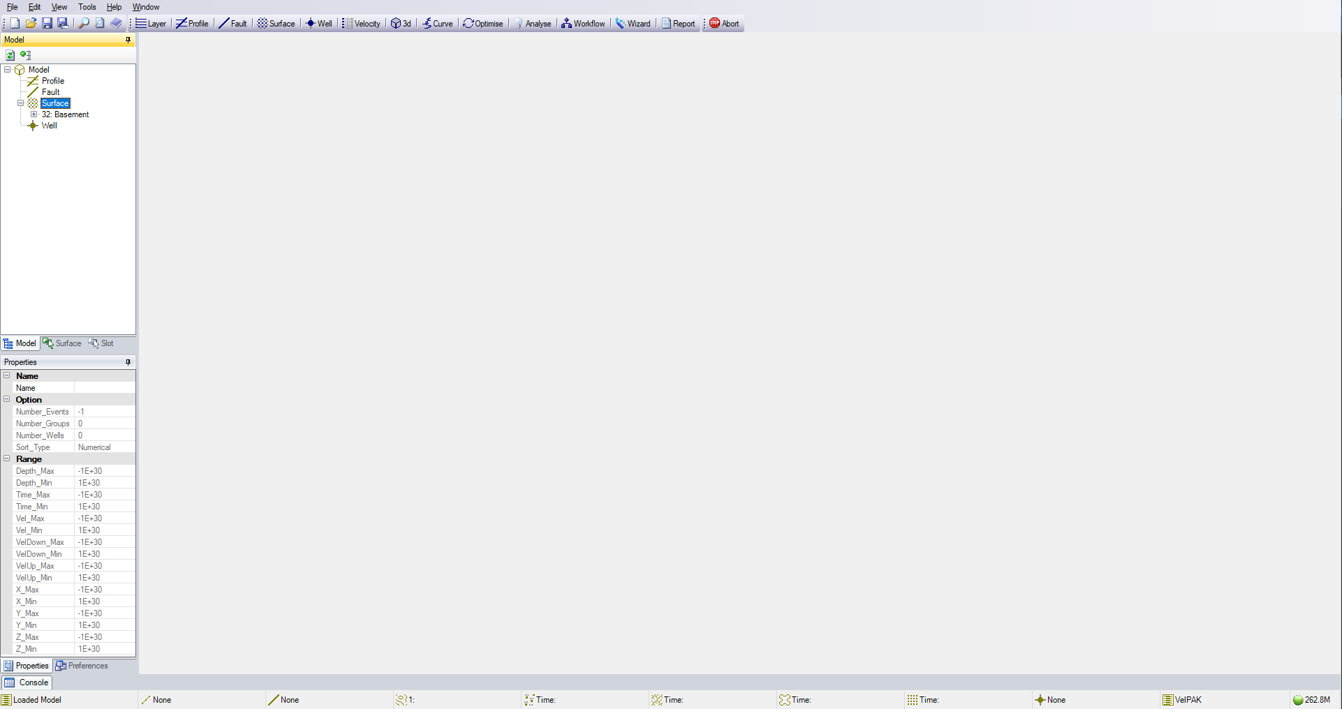
When you first open VelPAK, you are presented with a blank screen, with VelPAK having no data in it to work with, as you can see from expanding the model tree.
The first thing to do is to create a New model and save the file name. Due to the Windows character limit of 256 characters, it is essential that you place the model as close to the root of the hard disk drive that you are saving the data to. If not, you will likely crash the software.
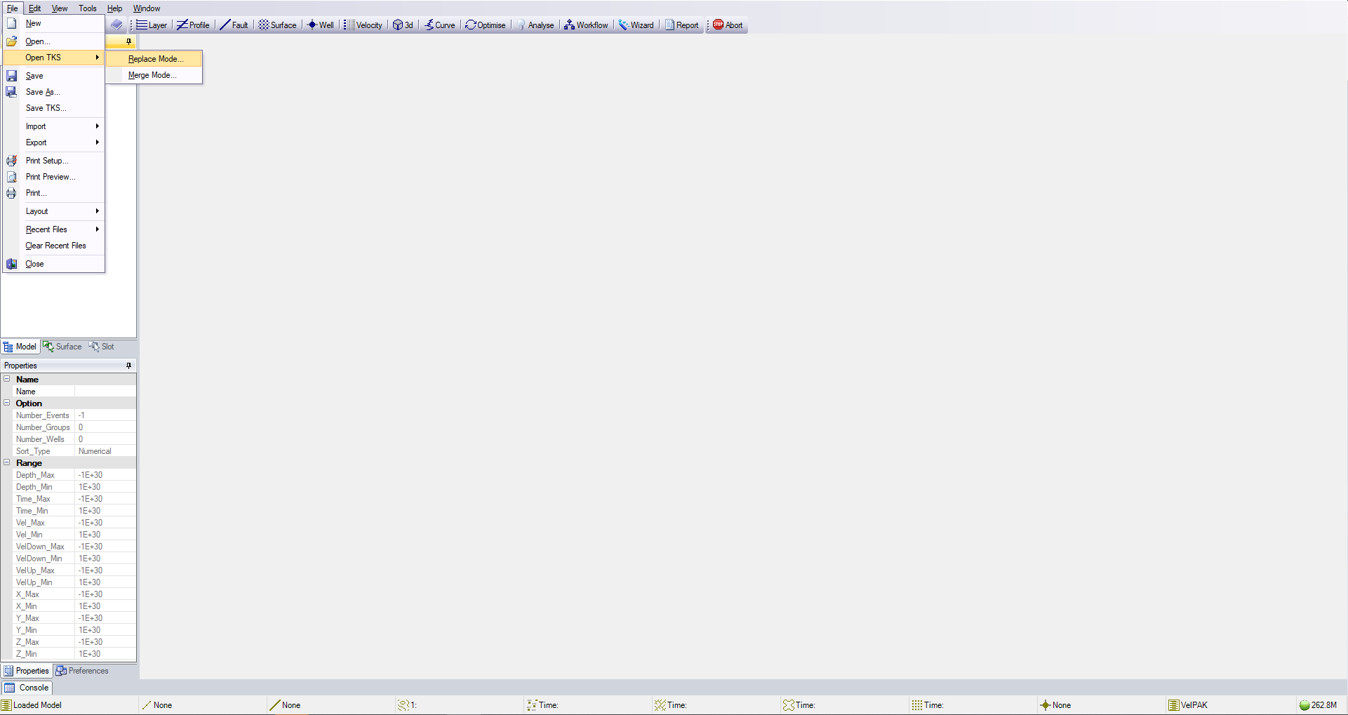
Next, select File > Open TKS > Replace Mode to open the Data Loading Wizard. (If you have already created a model and wish to add data to it, e.g. a new well, then you can select Merge Mode).
Data Loading Wizard
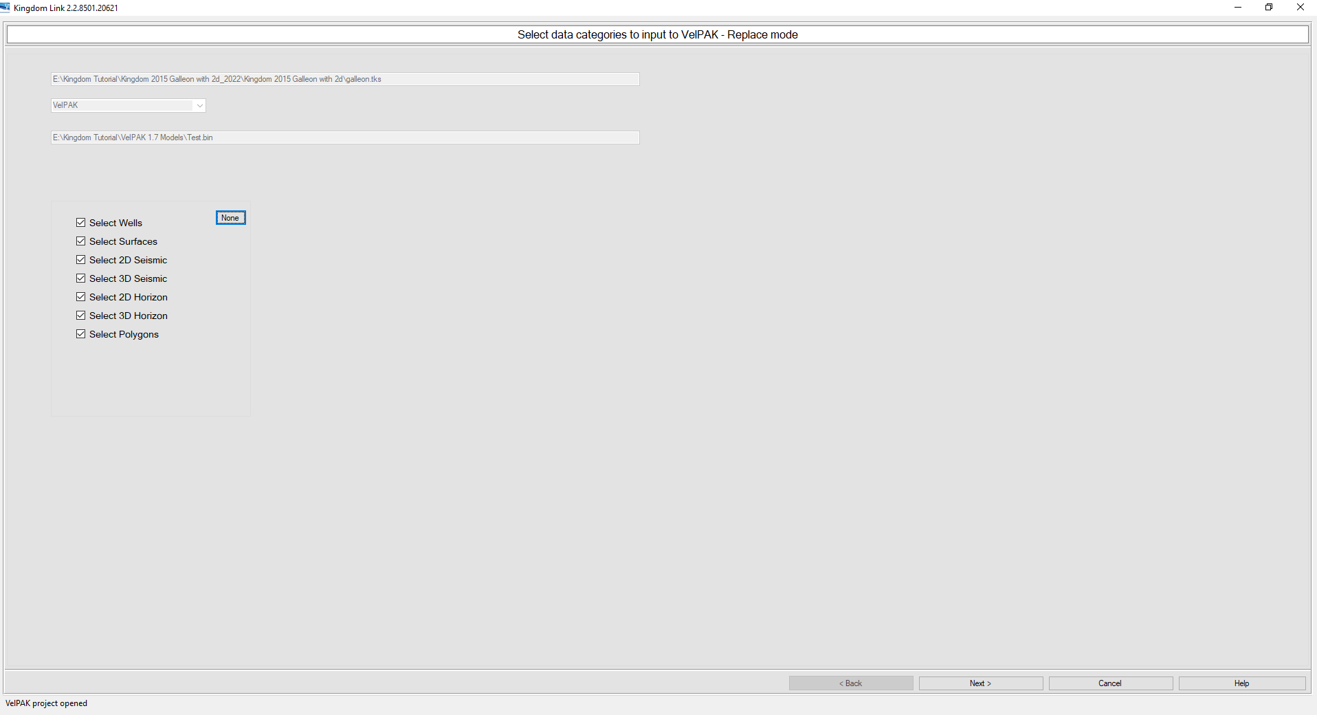
Upon first opening the Wizard, you are presented with the data selection screen. You can see the length of the parent folder of the Kingdom project and then the location of where the VelPAK model is stored.
Next, you can select the data you want to work with by clicking on the relevant tick boxes individually. Alternatively, you can click on the ‘All’ button to automatically tick all boxes.
Press Next to proceed to the following page.
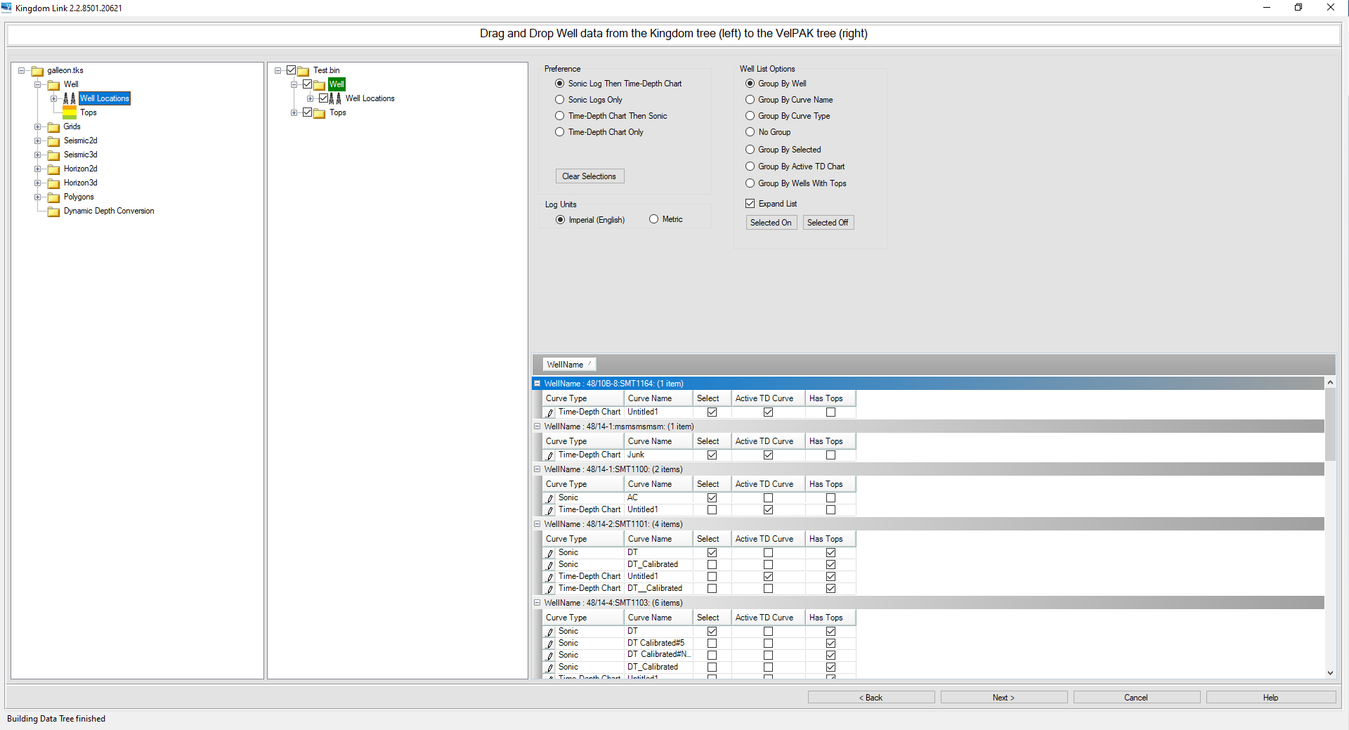
On this screen, you are prompted to ‘Drag and Drop Well data from the Kingdom tree (left) to the VelPAK tree (right)’. To complete this operation, left click on the Well Locations folder to highlight it in blue, then hold the left mouse button down and drag it over to the Well folder. This will simultaneously bring the tops over with the selection.
If you look to the right of the screen in the grey area, you can then preference the type of well data you want the software to work with. Typically, you’d preference the higher resolution Sonic Log data over the Time-Depth Chart data (as per the default option), but you can select any of the 4 options as per your preference.
You can then view the well data in different grouping arrangements and you can click on the relevant type to automatically reconfigure the display below, as per your selection.
Of note here, it is especially important for you to scroll through your wells and ensure that the tick box that is selecting the DT used in each well, is the one you want, as it is often the case that the default option is not the one you’ll want.
Once you have checked the relevant tick boxes and are happy to continue, press the Next button.
This page is where you will start to ‘build’ the model. The first step is to select the number of layers you want in the model by selecting this from the drop down menu in the centre of the screen.
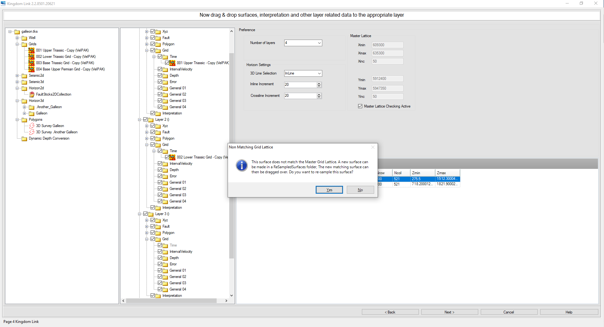
You then select the relevant time grids by left clicking on them, and then holding the left mouse button down to drag them into the Layer ‘n’ > Grid > Time folder. The first layer you choose will determine the Master Lattice used by the model in terms of the X and Y min/max coordinates. If any of your time grids do not conform to with the first layer, you will see the ‘Non Matching Grid Lattice’ dialogue appear. Pressing Yes will prompt the software to reformat the chosen time grid to conform with the coordinates of the first layer selected.
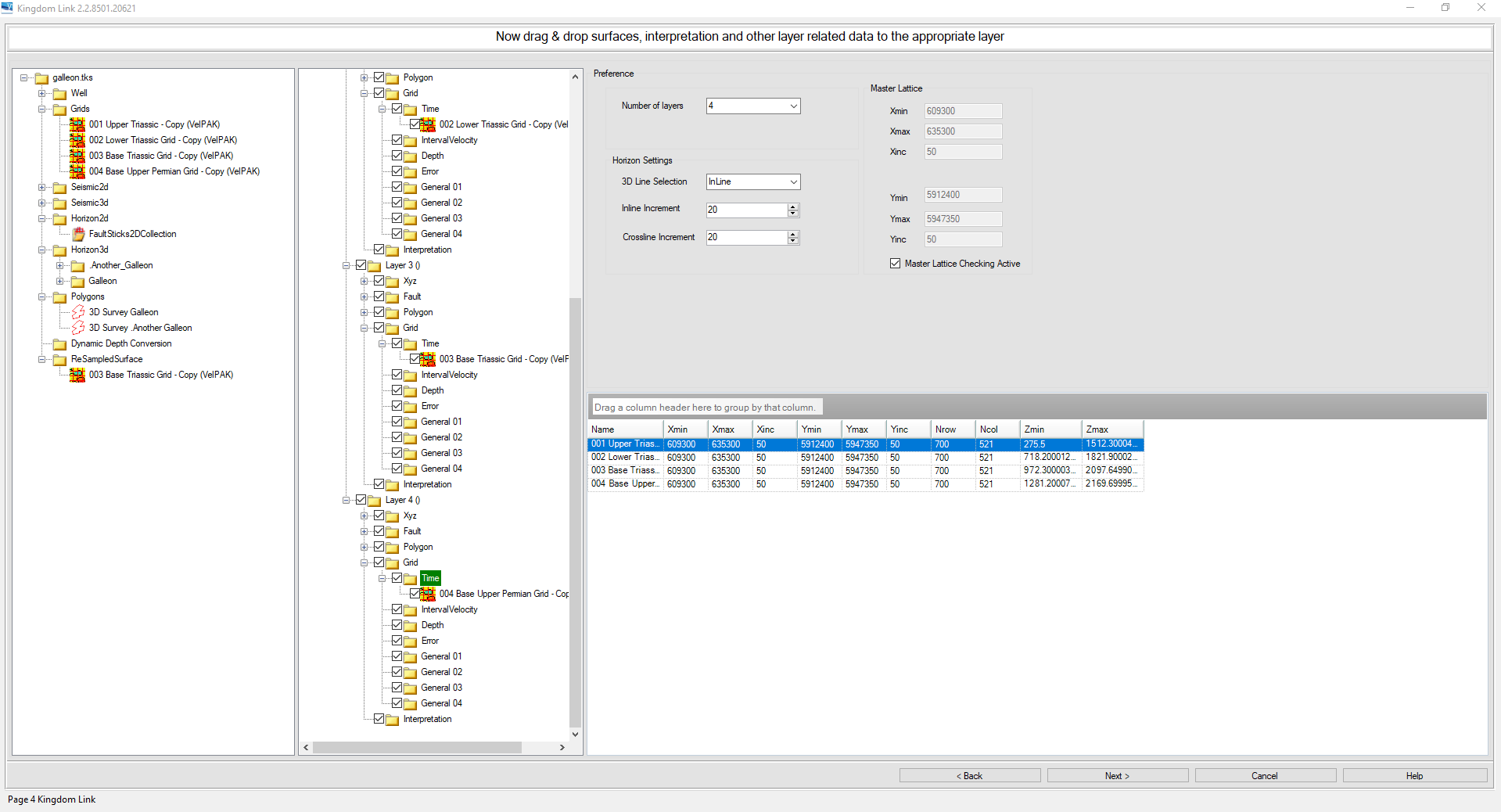
This surface is then available to drag and drop from the ReSampledSurface folder. Continue dragging and dropping your other time grids until all of them have been selected.
At this stage, you have the option to perform a similar process for your Fault Sticks and Horizon data if you are planning to use the software in the 2D profile mode. You can also drag across any polygons you’ve created in Kingdom that you want to work with in VelPAK. These are optional depending on your project objectives.
Once this step has been performed, press Next to continue.
This screen is where you get the formation tops and the time grids to correspond with one another. Here, you left click the formation top and then left click and hold to drag it into the folder ‘Tops in order of preference’ for the given layer. If you accidentally drag across the top into the wrong layer, you can right click to remove it from the list. You can also have the ability to use multiple aliased top sets.
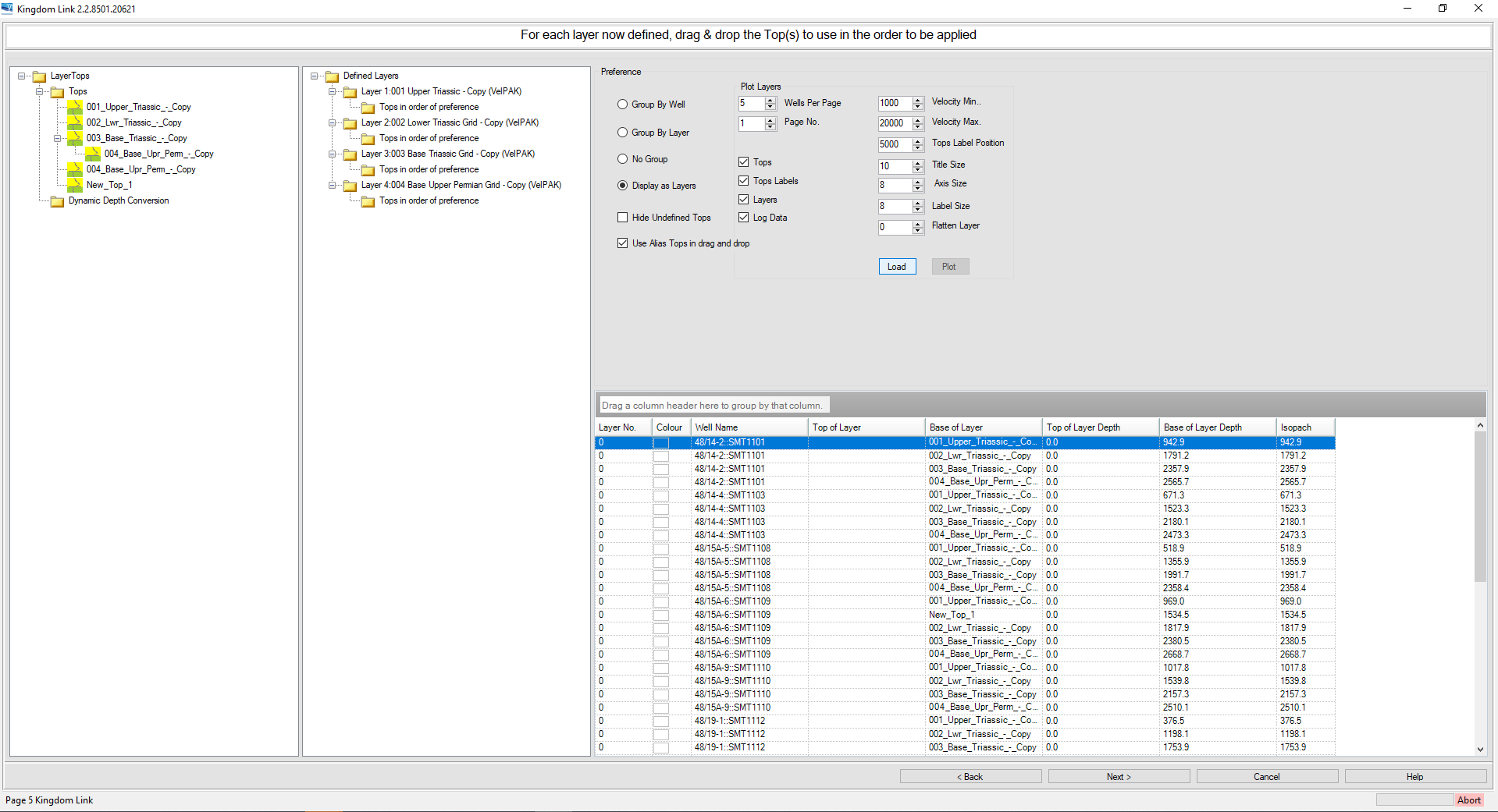
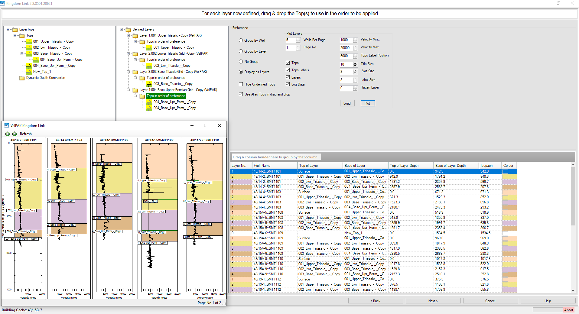
When you’ve completed this process, you can click on the Load button to see how the layer definition has been applied to the wells. You can then QC this in the table, where any wells that are missing information, such as there being an unconformity in the geological layering, will flag in red. You can select the top you want to use at the top of the layer in question, which will fix the red flag. After completing this step, you can click on Refresh on the display to update it.
When you have confirmed that the layering throughout your model is correct, press the Next button to proceed.
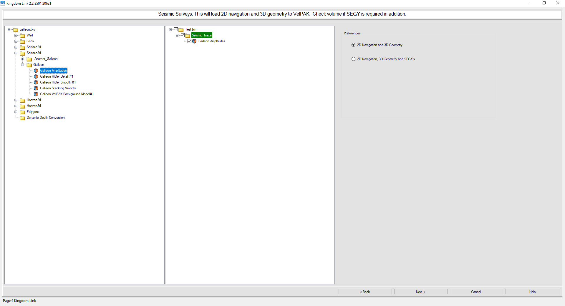
On this page, you can drag across the volume(s) you want to use for the geometry as well as numerous 2D lines. You can bring in as much data as you like here, but it should be covered the by areal extent of your time grids. This is an important step, as it loads all the coordinate information for the data into VelPAK, which will save you time in having to load it manually when you want to export an SEG-Y velocity cube as your end product of using the software.
Press Next to go to the following page.
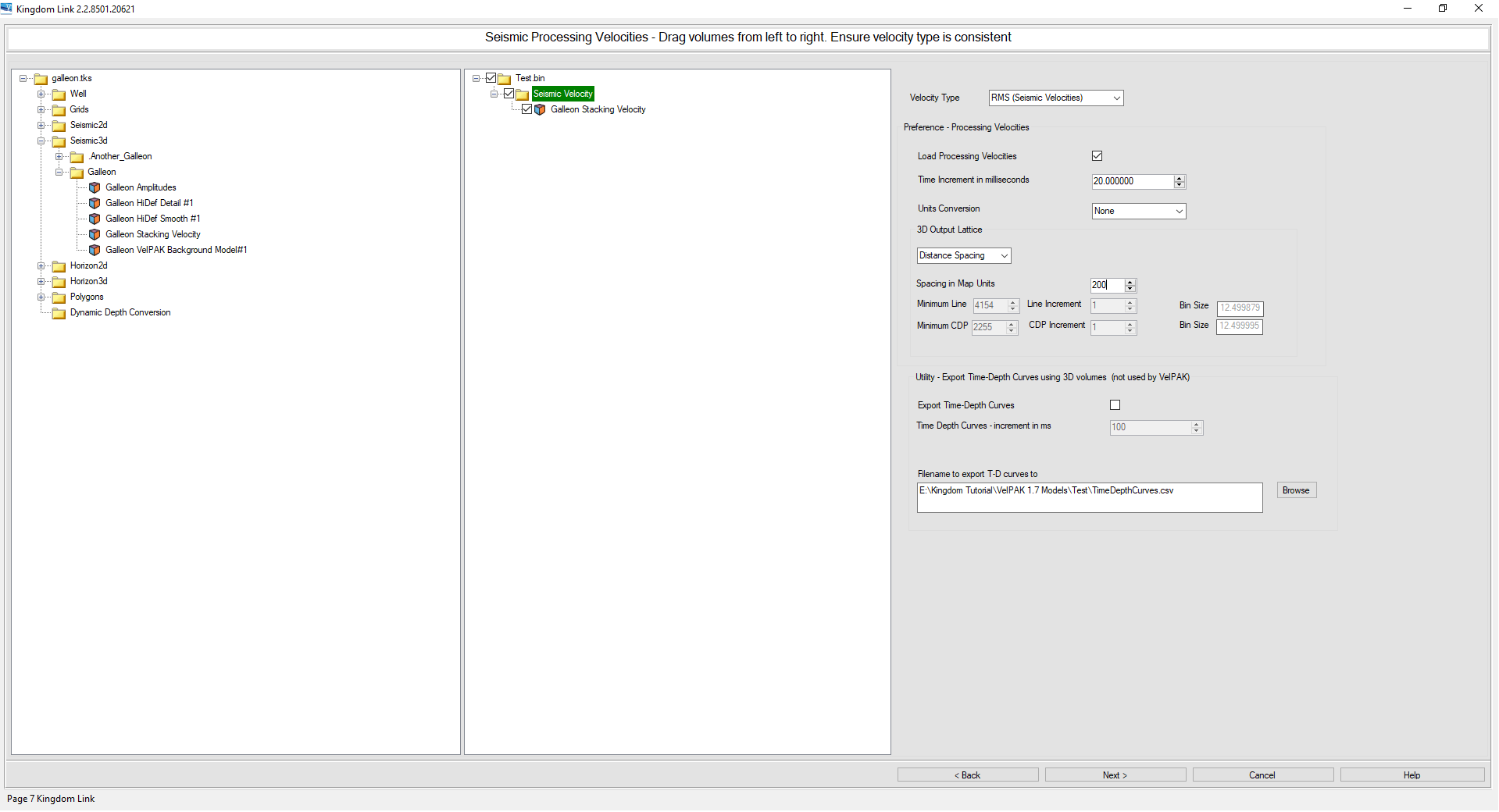
This page is where we select our Seismic Velocity volumes to work with in VelPAK. You can select the type of volume in the drop down menu, with RMS, Interval and Average options possible to load. The most important element here is to click on the tick box Load Processing Velocities. You can then choose the Time Increment in milliseconds. We would recommend using a vertical sampling over 10, with 20ms being suitable for most projects.
You can also specify the lateral spacing of points, with the units relating to metres or feet (as per the parent Kingdom project). If you look at the Bin Size of the data, it is recommended to select a lateral spacing value which is a multiple of the Bin Size. e.g. in this project the Bin Size is 12.5 metres and a lateral spacing of 200 metres has been chosen. One way to think of this is ‘how many data points do you want to sample from your velocity cube per kilometre?’
When you’ve selected an appropriate value to sample your volume by, press Next to continue.
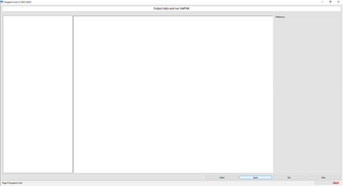
On this page click Apply to Output data and run VelPAK.
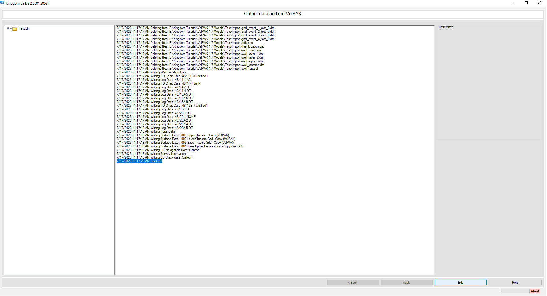
The software will take several seconds to load the data and will print its progress in the central window. When you see it say Finished! press the Exit key to load VelPAK.
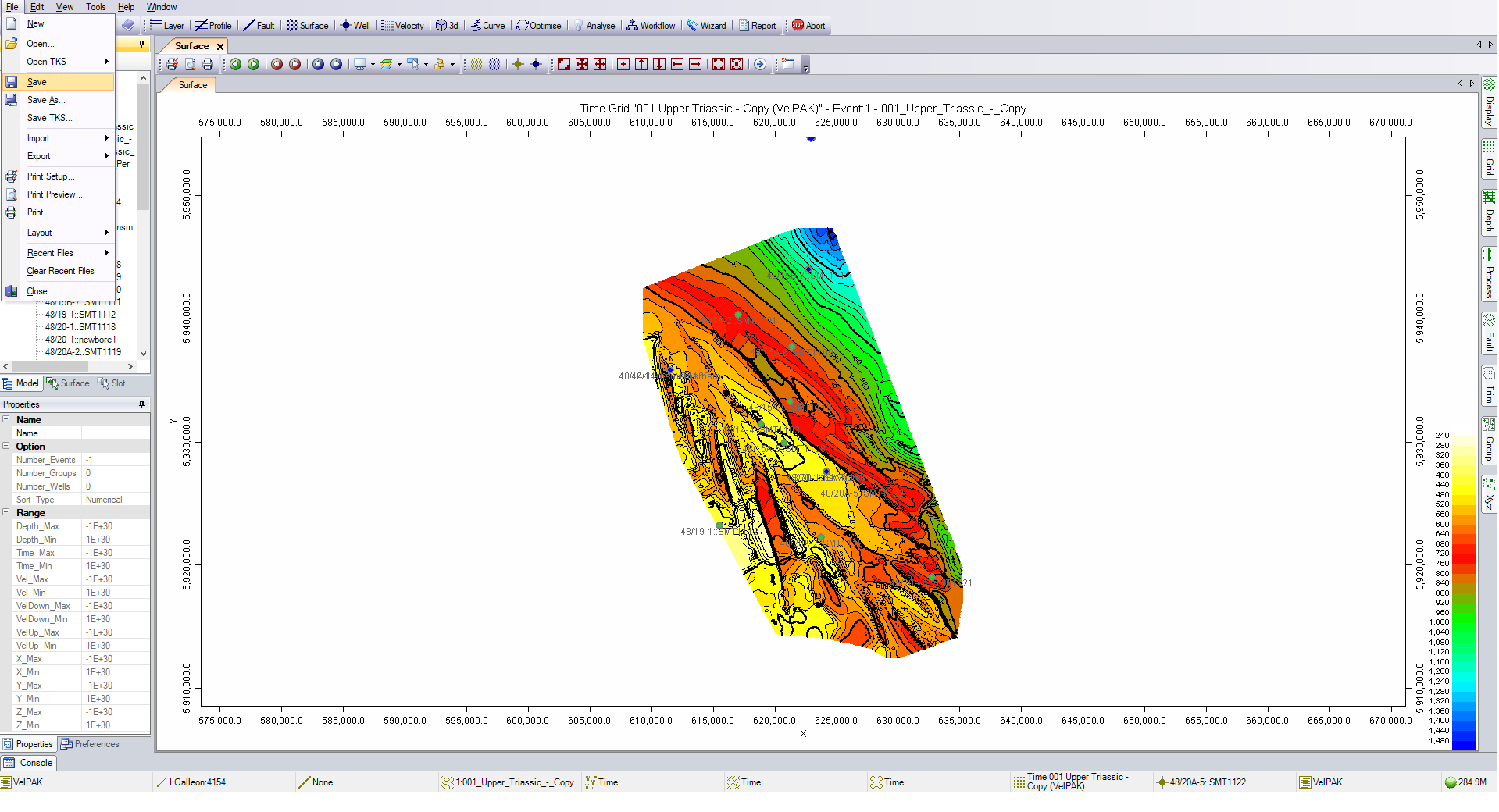
The data will now be loaded into VelPAK and you will be able to open the model tree to see the layers and wells. The most important step is to now press File > Save to update the save file of the model to include the data you just loaded. This will ensure if there is a power cut, etc, you won’t have to redo the data loading process.
We also recommend saving the model again under a different name, such that you can perform all your depth conversion work and always have to original data file as a backup if required.
If you would like to know more about Kingdom’s VelPAK (Velit on Petrel) then click here. Alternatively, you can contact us for a free evaluation by e-mailing us on sales@equipoisesoftware.com.
The software is provided by S&P Global (who we partner with for Kingdom) with perpetual and subscription pricing available on request. We offer a series of Teams meetings throughout the evaluation to help you quickly step up the learning curve and enable you to see the results for yourself.