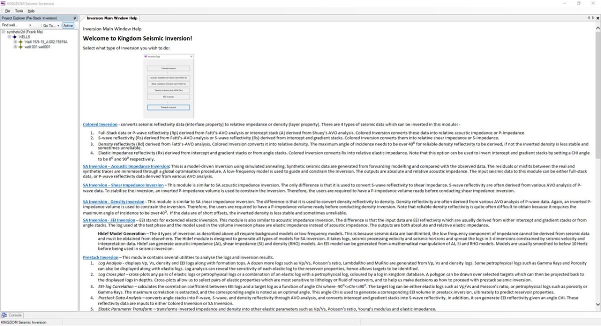
Upon loading Kingdom Seismic Inversion, you are presented with an initial selection screen where you can select the type of Inversion you wish to perform. At this first step, you can select ‘Prestack Inversion’ from the menu.
This option uses a cascaded Simulated Annealing workflow, such that you will first compute for the P-wave data, then take the output from that as the input for the computation of the S-wave data, followed by the output from that process as the input for the Density-data. This workflow has been designed so that you can output your final Pre-Stack attributes through a workflow that will typically take 5 working days to conclude.
Kingdom’s Pre-Stack Inversion has been designed to complement your existing Inversion portfolio by providing you with a ‘quick-look’ feasibility tool, which is easy to use and quick to run. This is in accordance with a ‘fail fast’ philosophy, and aims to enhance your operational efficiency. Using this toolset provides you with valuable information to make subsequent decisions, including enabling you to stick with the result, or use it as the basis for a continued workflow in other Inversion packages you might have in your software portfolio.
Data Selection Screen
You’ll find a model tree to the left-hand-side of the main window and this process is much like Colored Inversion and Simulated Annealing Inversion.
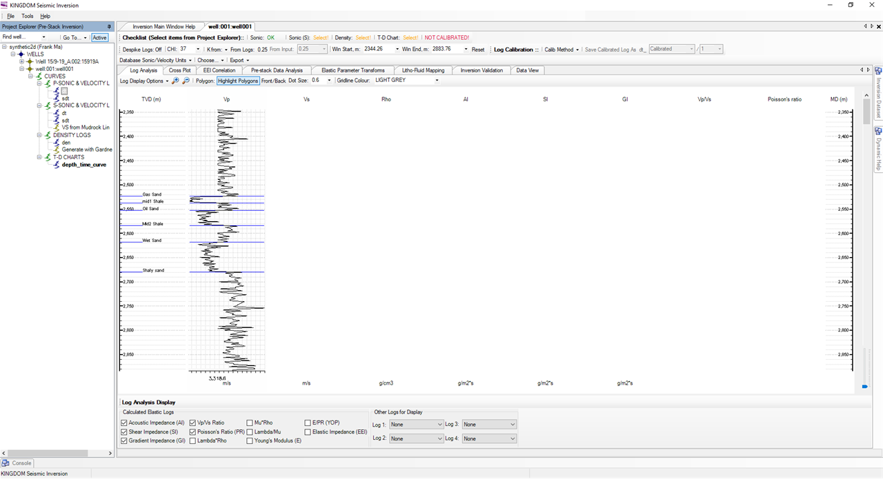
Firstly, select your DT, under Curves > Sonic & Velocity Logs. Then select your Shear-DT, then your Density Log, and then your Time-Depth chart. You can see that the panel which runs along the top of the screen will change from ‘Select’ to ‘OK’ with each successive click for the respective data types.
*Please note that the dataset used here is a synthetic data set provided by the University of Texas. This will make some of the visualisations very easy to separate the Gas, Oil and Water formations, which may not be the case in a ‘real world’ dataset.

Log Analysis Screen
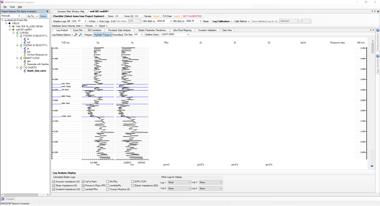
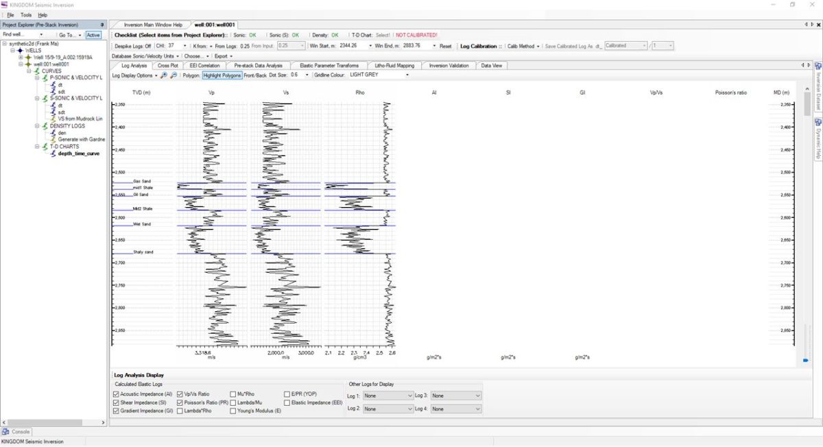
Once the 4 data inputs have been selected you can now click on the Log Analysis tab. In this window, the Vp, Vs, Density, Acoustic Impedance, Shear Impedance, Gradient Impedance, Vp/Vs and Poisson’s Ratio logs are shown by default. You then have the option to click the additional tick boxes to display several Lamda/Rho/Mu logs, Young’s Modulus and Extended Elastic Impedance logs. In addition, the software also permits you to visualise up to 4 petrophysical logs, such as the Saturation of Gas, Saturation of Oil, Porosity, Clay, etc. You can note that the formation markers are displayed in the TVD column on the left hand side of the display.
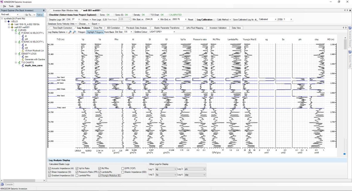
When you are happy with your selection, you can proceed to the Cross-plot tab.
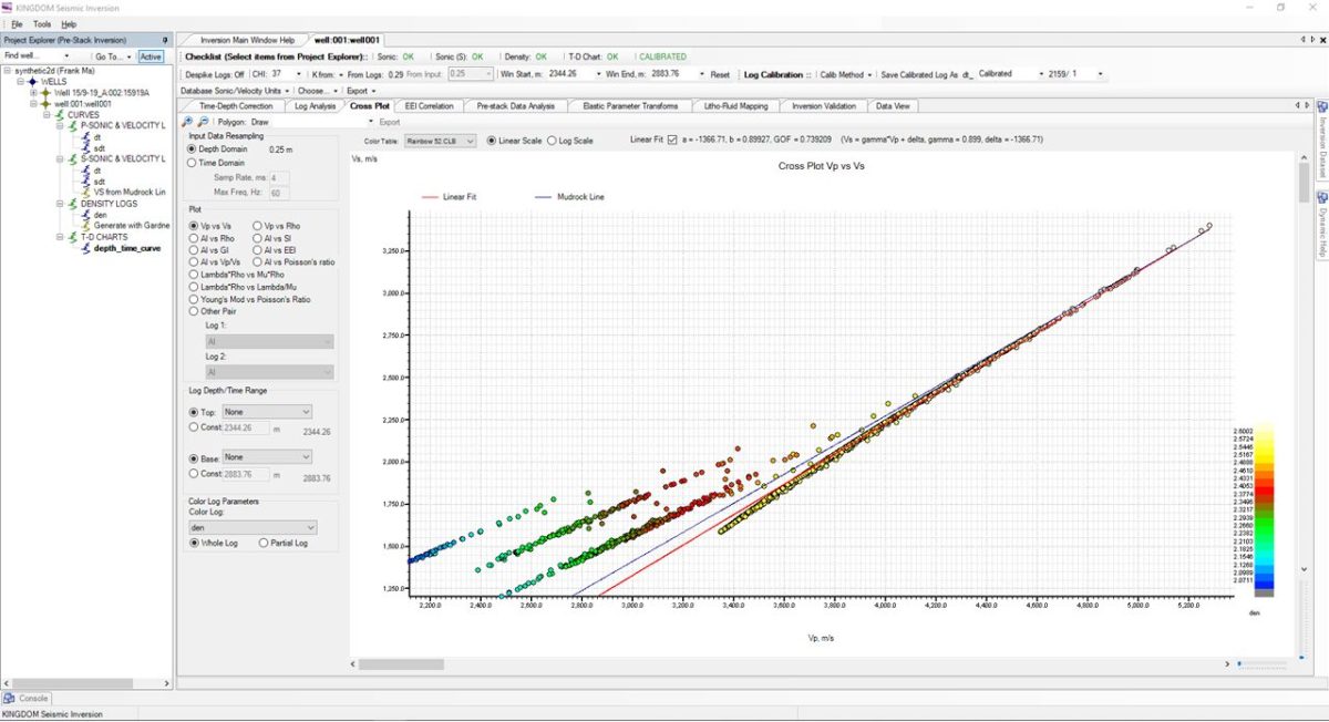
Cross-Plot Screen
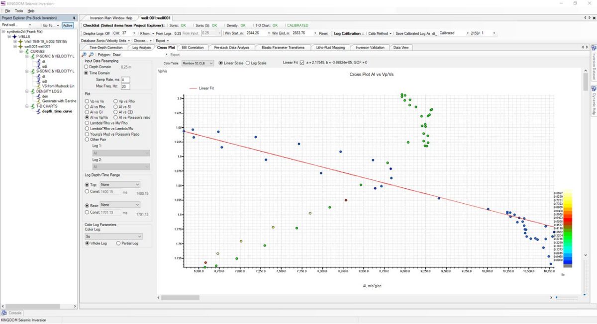
This screen has been designed as a feasibility tool to enable to see what your data can tell you (or not). It contains 11 industry standard plots as well as the ability to plot any X-axis vs any Y-axis, giving you the ability to interrogate your data from different perspectives. You can also specify the data range between a Top event and a Base event, or constrain the display by using a constant for the Top, and a different constant value for the Base events. You then have the option to select the dropdown menu and select the colour-fill of the data points to correlate with any of your petrophysical logs that you have present in Kingdom.
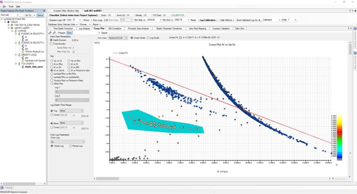
In the image below, the AI vs Vp/VS plot has been selected and the Saturation of Oil log has been selected as the colour bar, turning all the data points that relate to that property a different colour (in this instance the dots have turned white). You can then draw a polygon around these data points and click back on the Log Analysis tab to visualise where this property occurs in the logs.
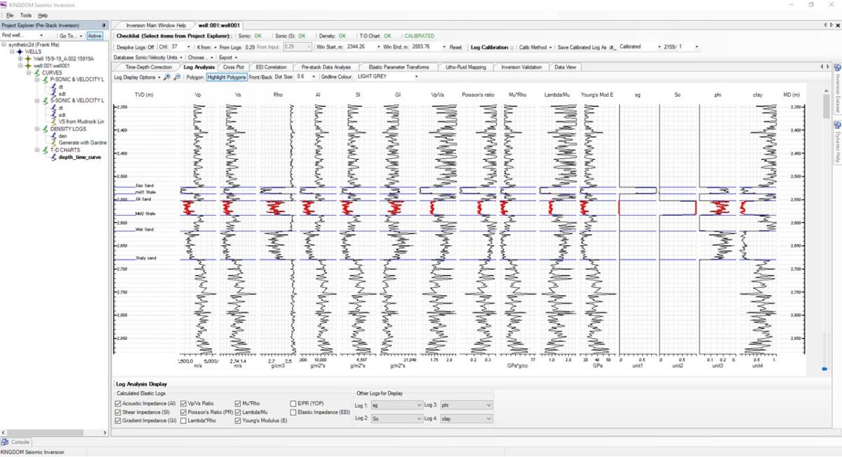
As you can see from this display, all the data points which relate to the presence of oil in the data are highlighted by a series of red dots plotted on the logs. You can repeat the above step for both gas and water to get a complete understanding of the different fluids contained in the reservoir.
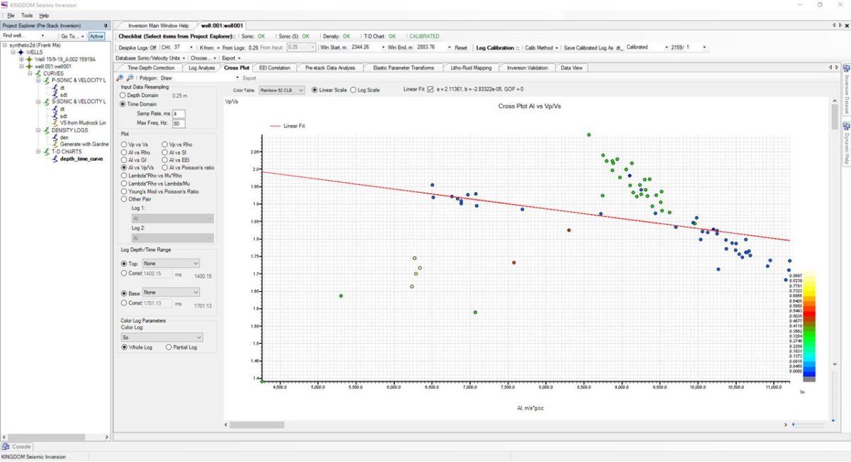
As part of your feasibility assessment, you can also plot the data in the time domain as a function of the sampling rate (in milliseconds) and the frequency of the data (in Hertz). As you can see from the two images below, at 20 Hz, it might not be possible to properly discern any fluids within your area of interest. This is due to the low number of sampling points. However, at 80 Hz, the reverse may be true. Either way, this tool will allow you to quickly understand what is permissible, or not, with your data.
Once you have completed your feasibility study, you can move onto the EEI Correlation tab.
Extended Elastic Impedance
This screen has been designed to allow you to determine the corresponding CHI angle at which your data can be rotated to predict different petrophysical logs. The red curve to the bottom left shows the maximum positive and negative peaks that correlate with a specific CHI angle. The middle window, and light green curve is a plot of the EEI Log at any given CHI angle. The plot to the right hand side is this log plotted against a given petrophysical log. In this example, porosity.
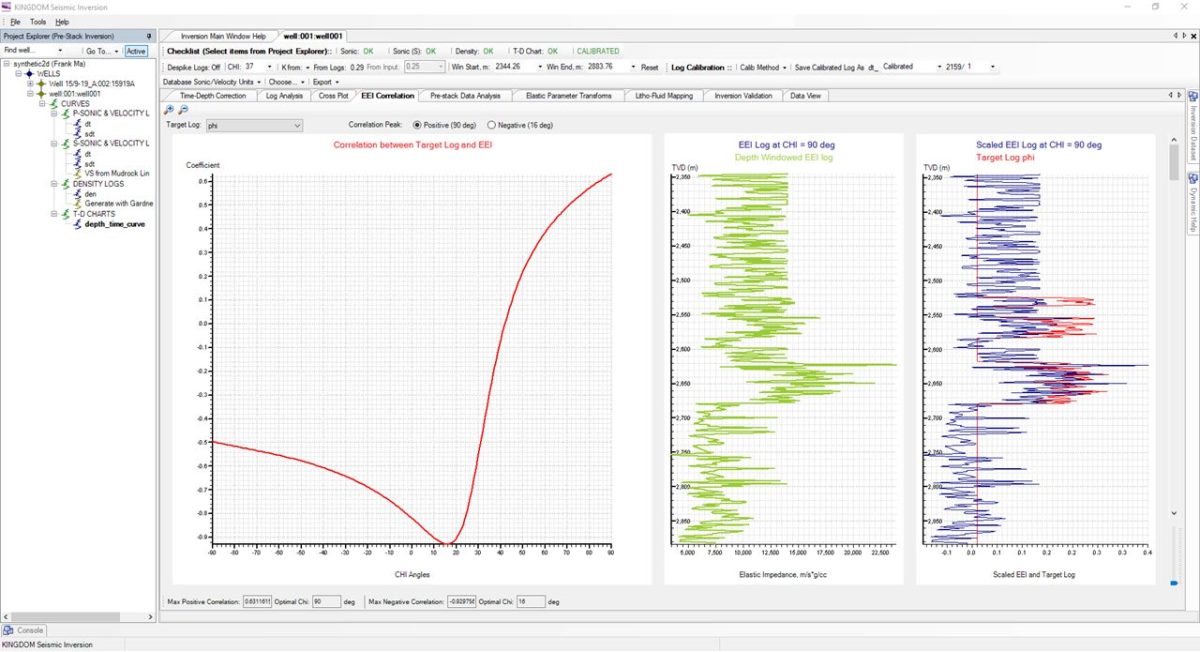
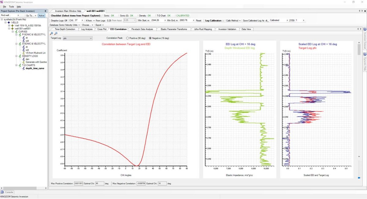
You can see in comparing the image above and below, by changing the correlation peak from Positive (30 degrees) to Negative (16 degrees) that in this instance, the CHI angle of 16 degrees provides a much better match to the Target Log of porosity. You can then repeat this process and determine the most suitable CHI angle used to predict any given petrophysical parameter and note them down for use later in the workflow.
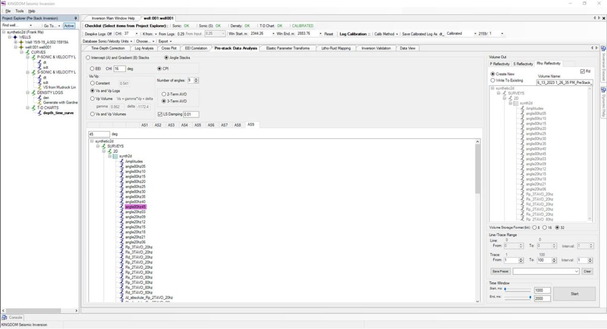
Pre-Stack Data Analysis
On this tab, you are able to generate reflectivity volumes based on your available data as inputs. Firstly, you can use your Intercept (A) and Gradient (B) stacks and use this to generate a P-Reflectivity volume. Alternatively, you can use your Angle Stacks and 2-Term AVO to generate both P and S-Reflectivity volumes, or if you have long offset data with angles over 40 degrees you can generate P, S and Density (Rho) Reflectivity volumes. To add these, simply increase the number of angles (to a maximum of 9) and correlate each angle (AS1 – AS9) with a corresponding file in the tree below, while also editing the angle in degrees in the box at the top of the tree. On this page you can also enter if your EEI CHI angle and generate a volume of that property.
This page presents you first time that you’ll need to have the computer spend time processing the data. On an average sized dataset, it would typically take about 2 hours to process each volume. You can choose to perform more targeted processing by selecting the line trace range, as well as the time window. When you are ready, click the Start button to commence the process.
Cascaded Pre-Stack Inversion
When the Reflectivity volumes have been computed, you will then select Tools > Acoustic Impedance and perform a Simulated Annealing inversion using the P-wave volume as your input. Typically, this may take 8 hours or overnight to process. Next, you’ll repeat the same workflow, but use the S-wave reflectivity volume as your input, using Tools > Shear Impedance, which will take a similar amount of time to process. Finally, you’ll use the Density reflectivity volume as your input to the Tools > Density option and run thorough the Simulated Annealing steps to generate that volume.
If you imagine the workflow so far:
Day 1 = Feasibility Analysis and Reflectivity Volume Generation
Day 2 = AI Volume Generation
Day 3 = SI Volume Generation
Day 4 = Rho Volume Generation
And so we come to Day 5 of our workflow to complete the final steps:
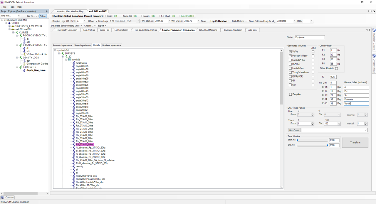
Elastic Parameter Transforms
You now come back to Tools > Pre-Stack Inversion, select the 4 data types to continue and skip to the Elastic Parameter Transforms tab. Here, you can use the inputs of your Acoustic Impedance, Shear Impedance, Density and Gradient Impedance (if generated earlier) to generate a number of different volumes such as Vp/Vs, Poisson’s Ratio, etc. You can also generate the Relative Impedance volume of each of the primary volumes that you’ve selected, and use an Ormsby Filter as part of this process. In addition, on this page you can create up to 5 CHI angle volumes and provide each with a volume label.
When you have your selection complete, click Transform to start the process. But, be aware that for each volume you tick to select, you can quite rapidly burn through your hard disk space!
This process should take about 30 minutes per volume to complete.
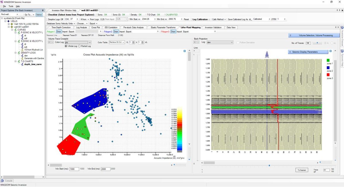
Litho-Fluid Mapping
On this tab, the first thing to do is select the property you want to plot on the X-axis and Y-axis respectively. In this instance, the Acoustic Impedance volume has been selected for the X volume In and the Vp/Vs volume has been selected for the Y.
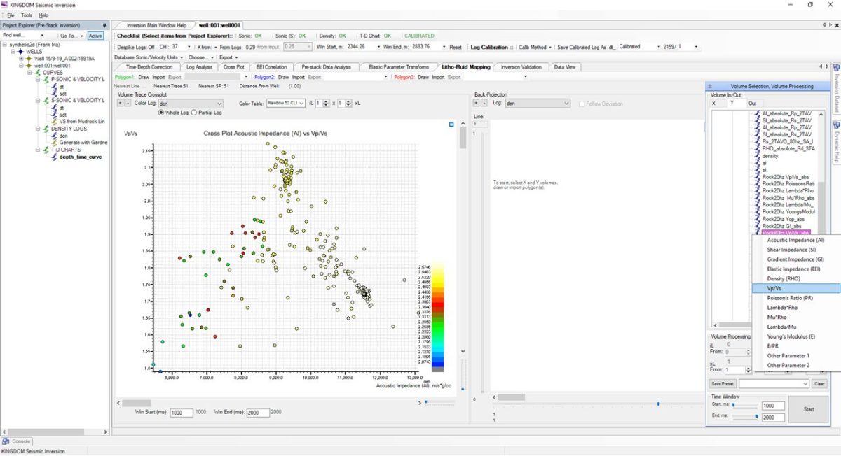
Next, you can change the Color Log to be, for example, your Saturation of Gas log and then draw around those data points in red. Then, you can change the Color Log to show your Saturation of Oil log and draw around those points in green.
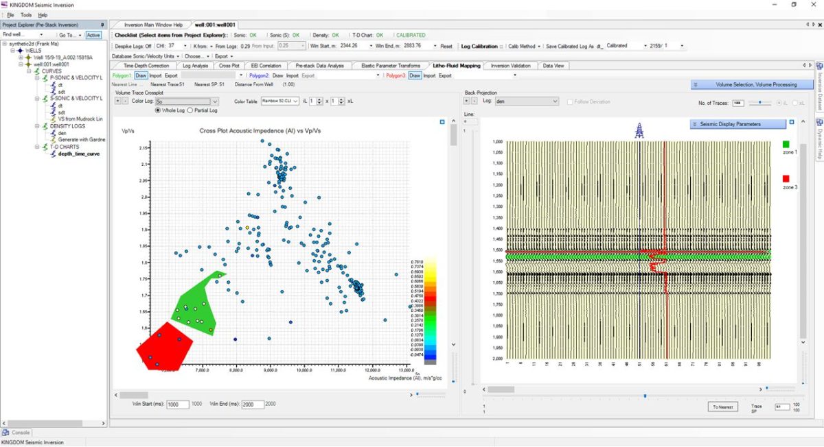
By selecting the porosity log, you can discern the data points which correspond with the presence of a wet sand, and fully differentiate the fluids contained within your reservoir.
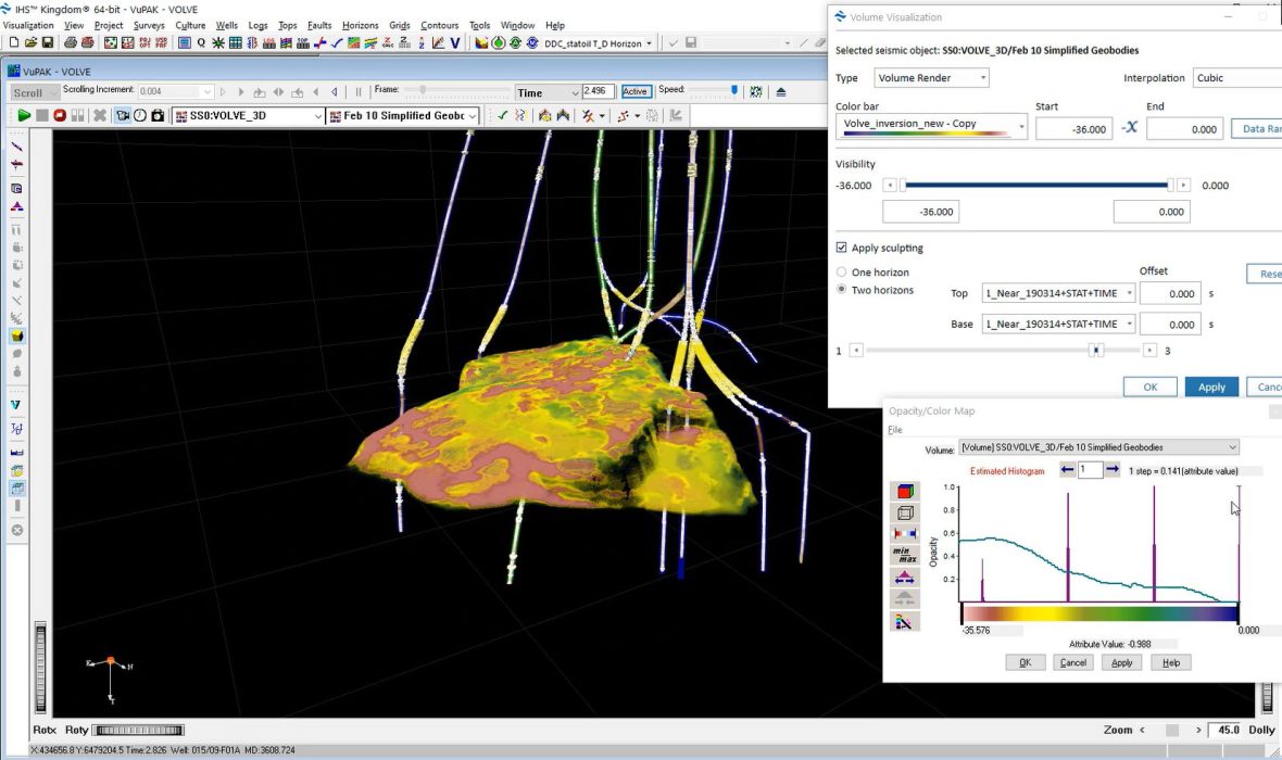
You can then output a volume containing all the data points sorted into their fluid type; gas, oil and water and load this into Kingdom’s VuPAK module.
View The Results In Kingdom
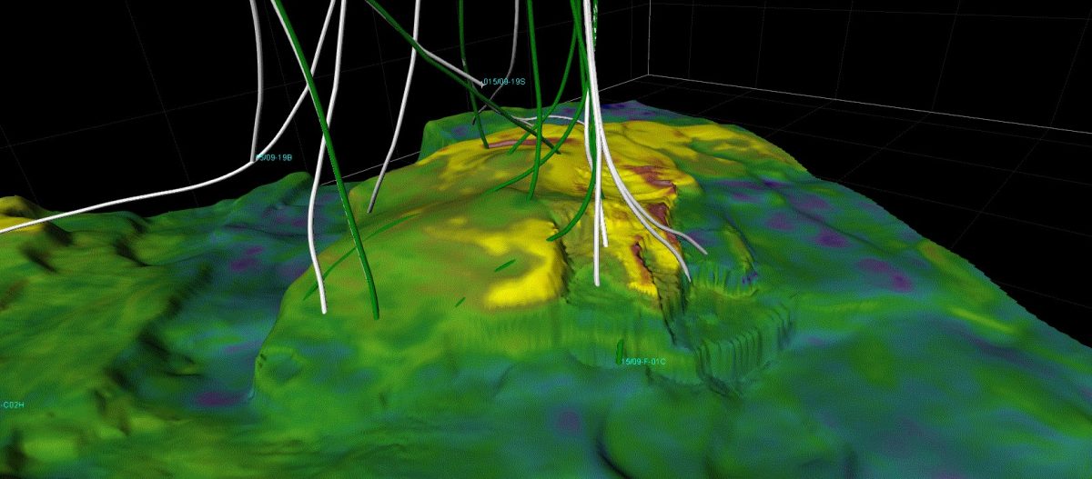
The final step would be to use Kingdom’s sculpting tools to remove the background geology from the 3D visualisation, and just view the reservoir filled with each of the 3 fluid types. The colour scale here denotes gas as being red, oil as yellow and water as green/blue.
The result is a workflow which is easy to apply, will take you approximately 5 days to complete and will provide you with a cost-effective end result which can serve as your final product, or one in which you can utilise as your starting point for another inversion method in another software package.
If you would like to maximise the value of your seismic data and leverage additional pre-stack attributes to improve your data interpretability or if you’d like to know more about Kingdom Seismic Inversion then click here. Alternatively, you can contact us for a free evaluation by e-mailing us on sales@equipoisesoftware.com.
The software is provided by S&P Global (who we partner with for Kingdom) with perpetual and subscription pricing available on request. We offer a series of Teams meetings throughout the evaluation to help you quickly step up the learning curve and enable you to see the results for yourself.