This article covers the steps to perform kriging with external drift as a method of depth conversion for any given layer in your layer cake velocity model. You should note however, that this technique is robust primarily for layers with flat geology and low geological complexity, as this process is going to map the vertical apparent interval velocities to provide you with a depth grid that encompasses lateral velocity variation, but has no vertical velocity component.
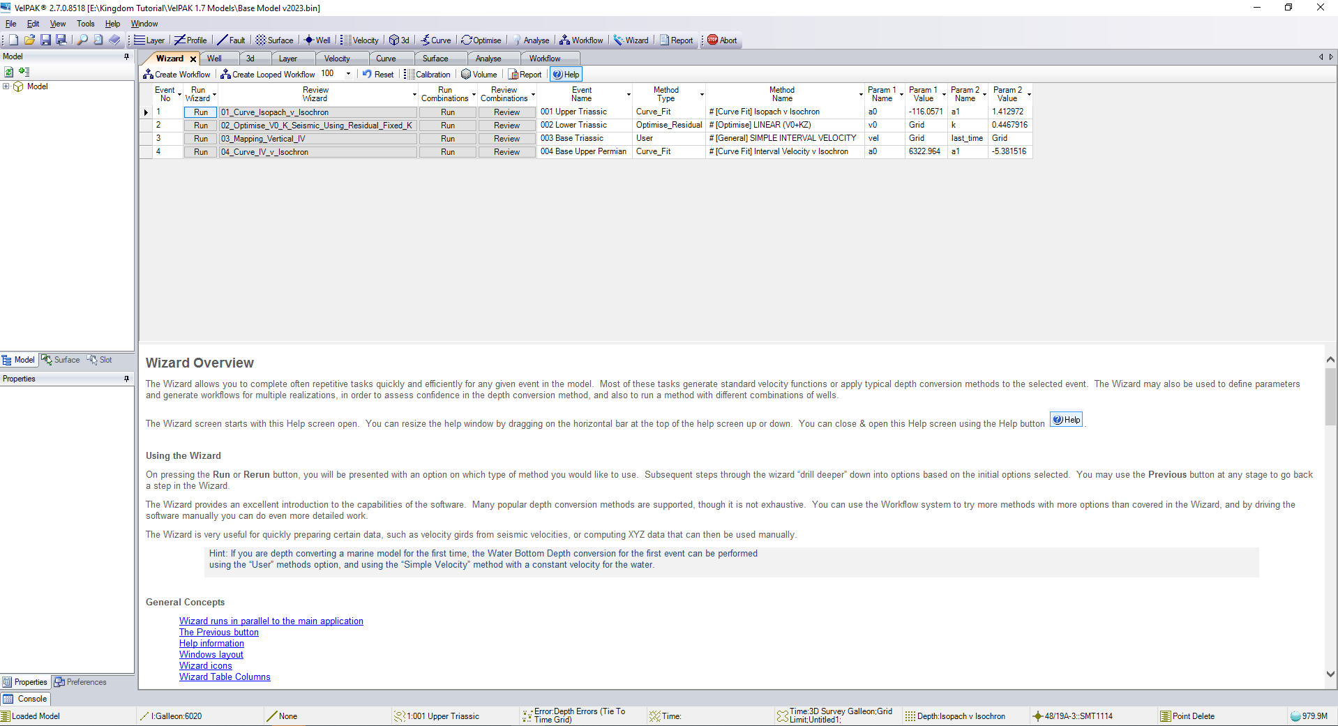
We start in VelPAK’s Wizard module and select the layer you wish to perform this technique on. In this example I am selecting Run on Layer 1.
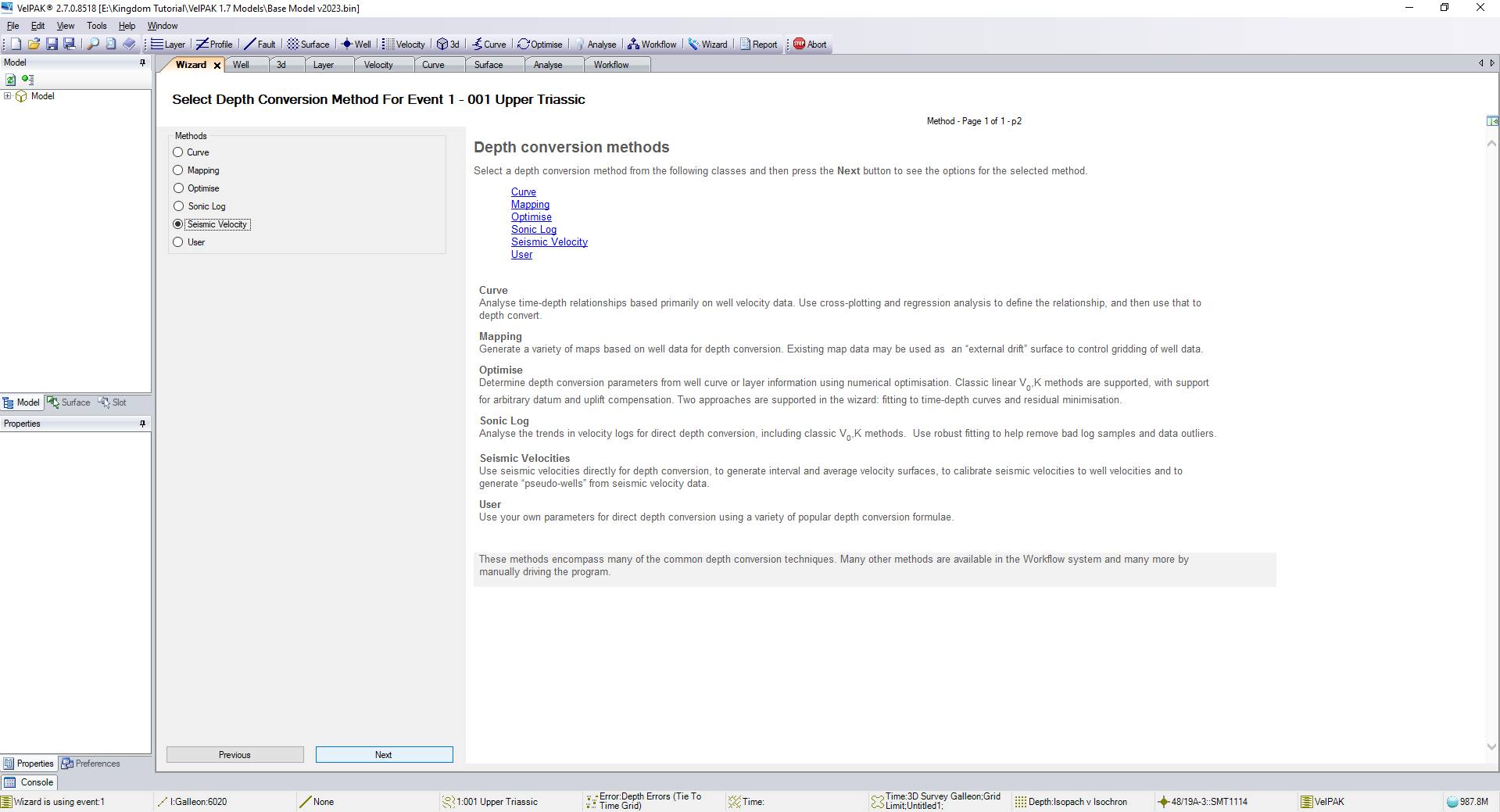
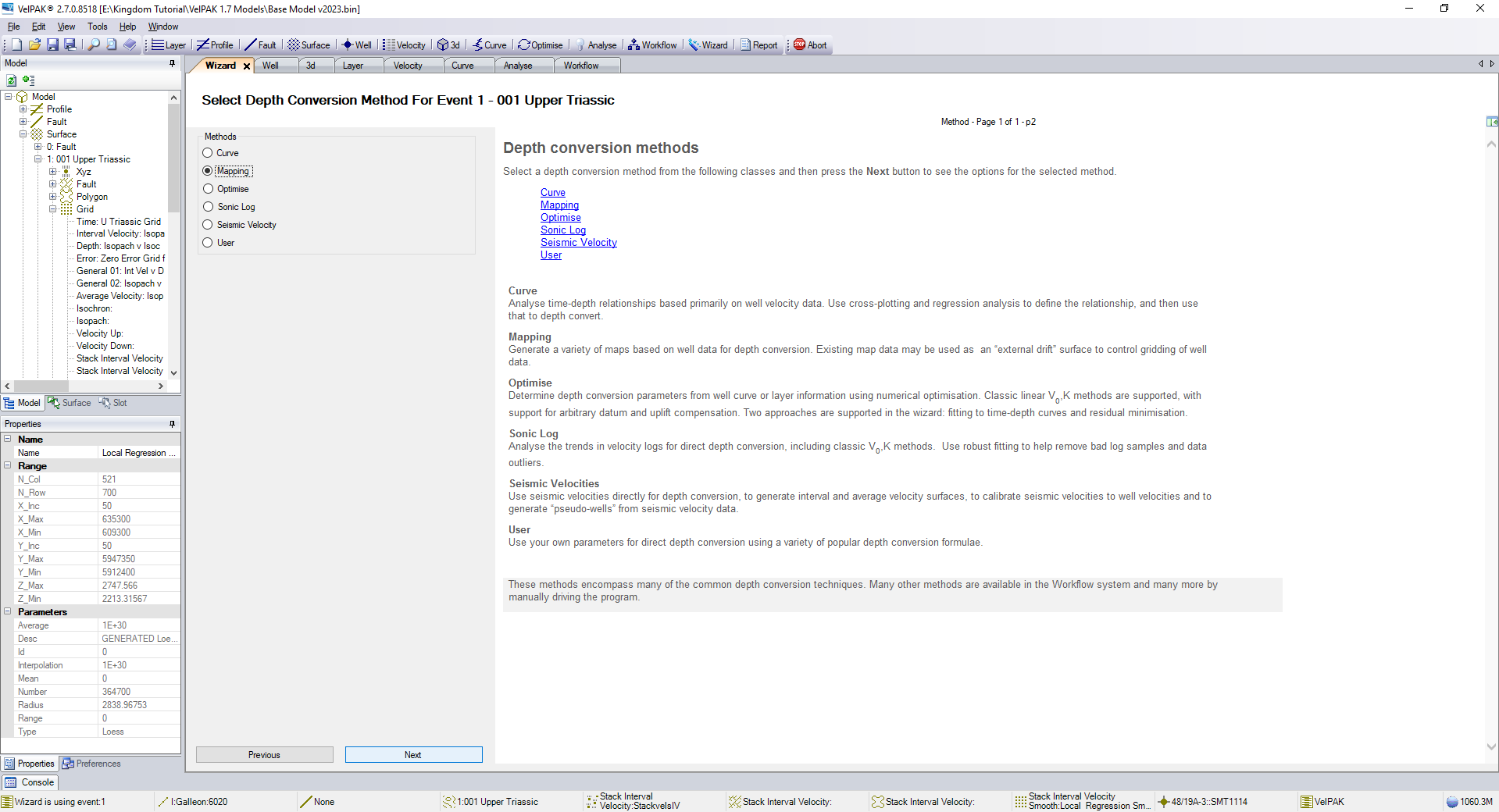
You then select the option of Seismic Velocity and press Next.
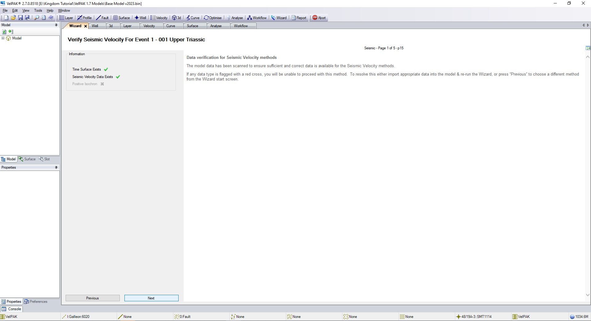
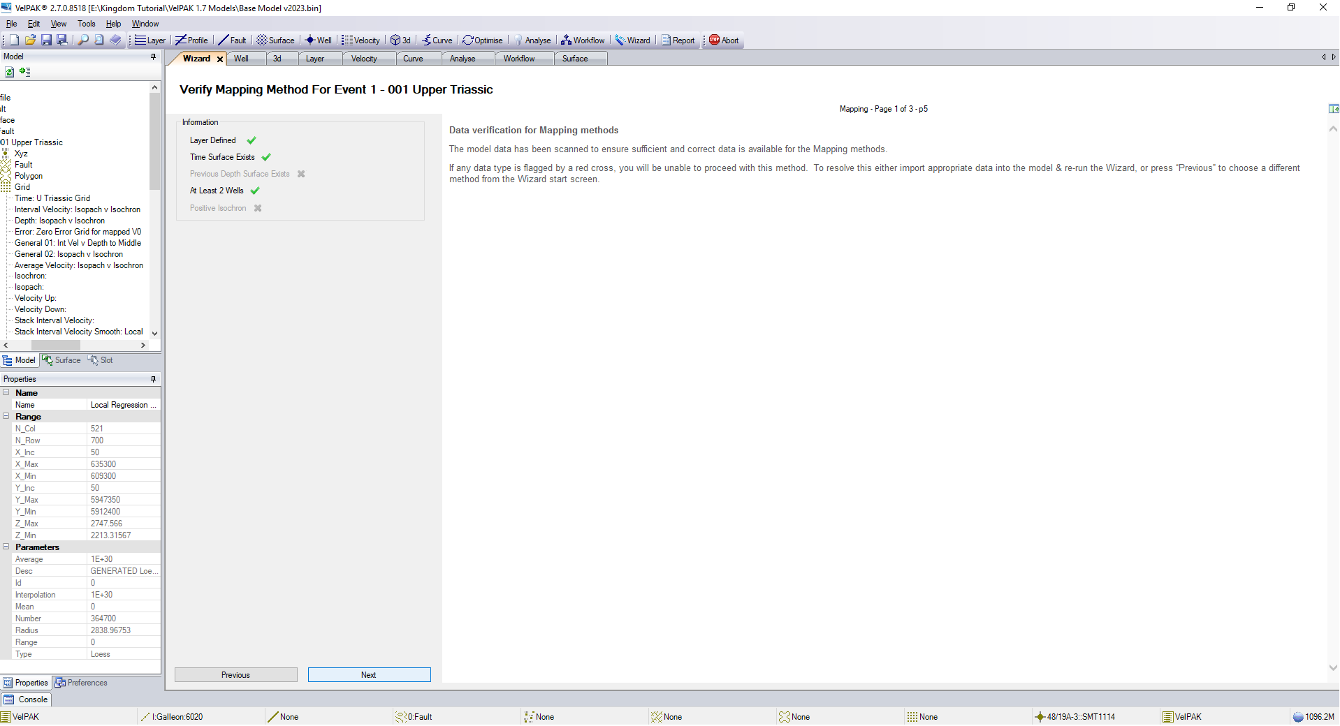
The software will check that you have the data loaded into the model you’re working in and show you the green tick marks to confirm everything is OK. If there is a Positive Isochron for a given layer, the software will provide you with a button called ‘Fix’ which will automatically edit the grid to conform with the overlapping surface. If everything is in good order, press Next to proceed.
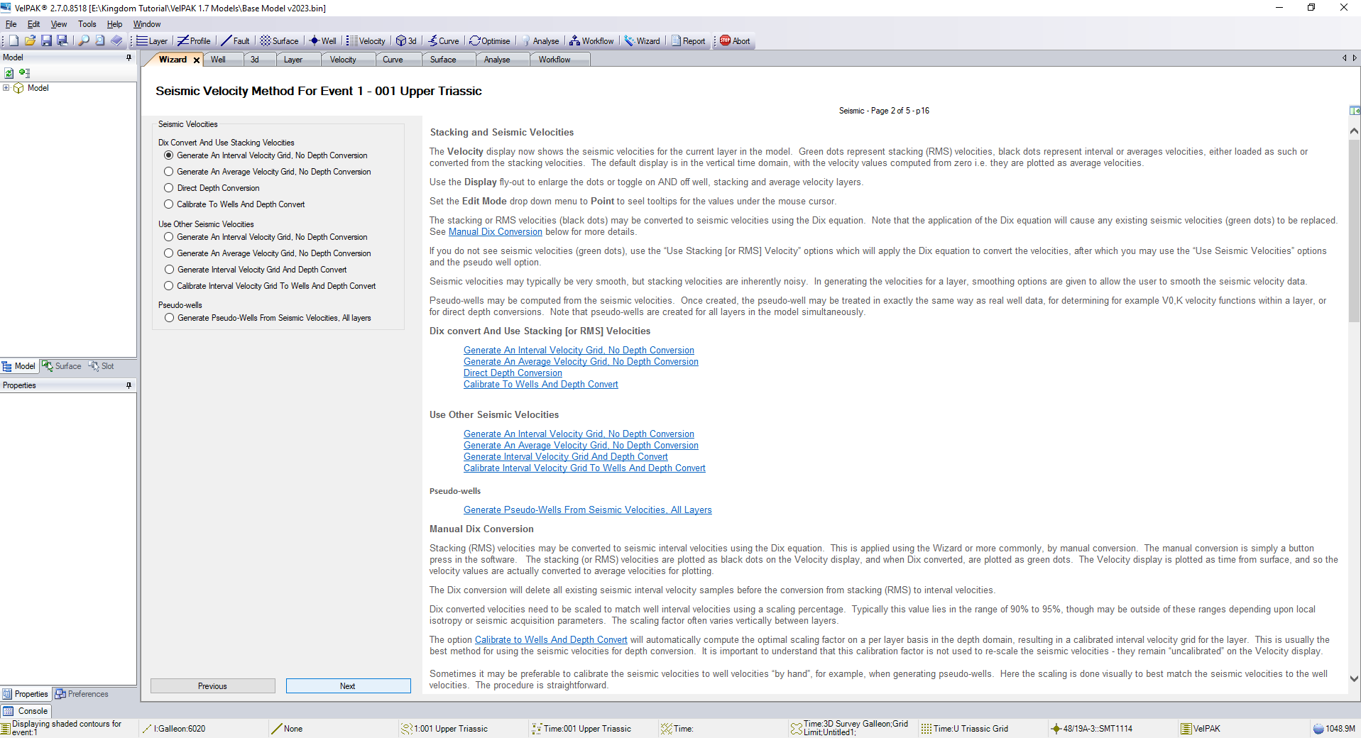
On this screen you are presented with many options for working with Seismic Velocities. If you have an RMS volume, you can select the top option, which will Dix convert the velocities. Alternatively, if you have loaded an Interval or Average velocity volume, you can select the option under “Use Other Seismic Velocities” to Generate An Interval Velocity Grid, No Depth Conversion. When you have made either selection, press Next.
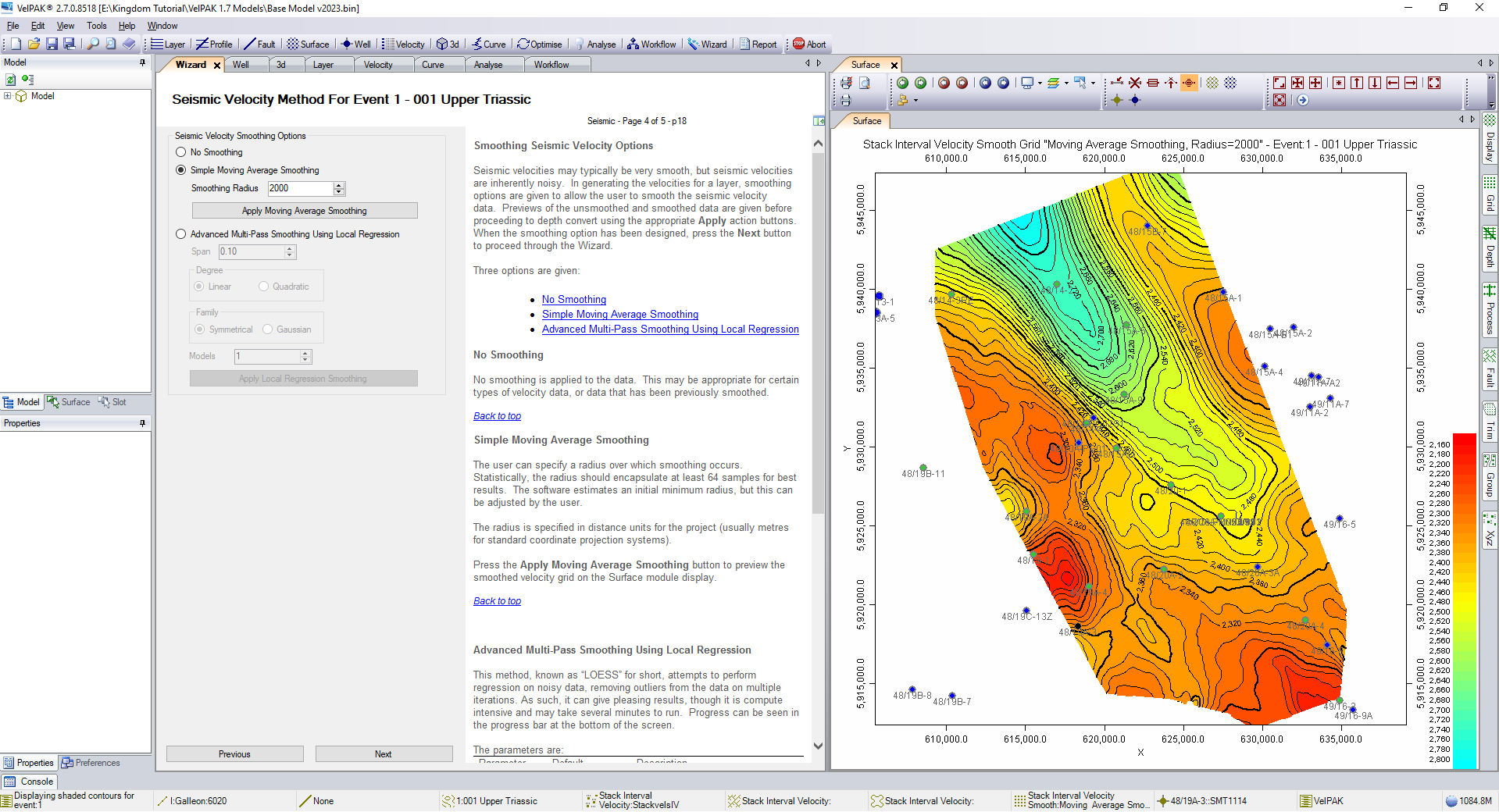
On this page you are presented with 2 options to perform a smoothing operation on your data. Before doing this, you should dock the Surface tab to the side of the Wizard, so that you can see both modules as illustrated in the example below. The first option is the Simple Moving Average Smoothing, where you can set the radius (with this number relating to feet or metres depending on your project units) of the degree of smoothing you want for the grid.
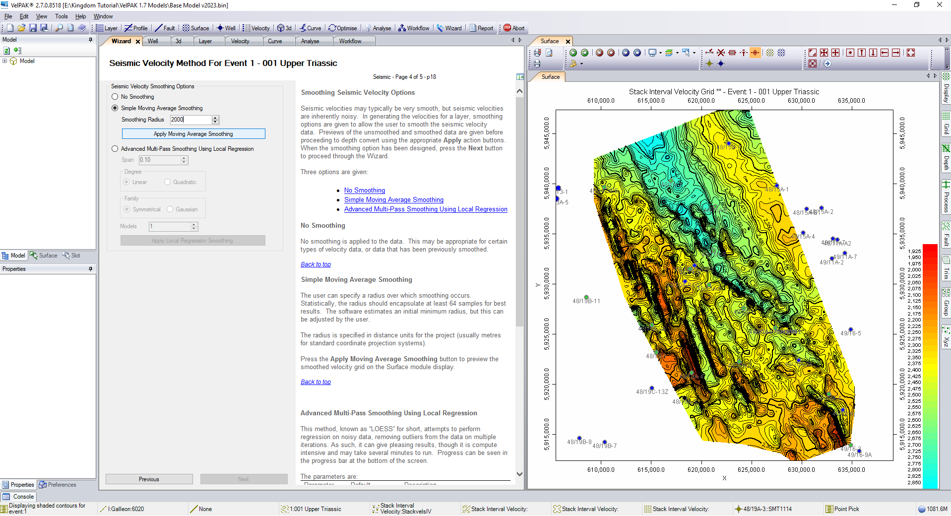
In this example the value of 2000 metres has been used, but this is an arbitrary value and can differ depending on the size of your survey area and how smooth you want your grid to be.
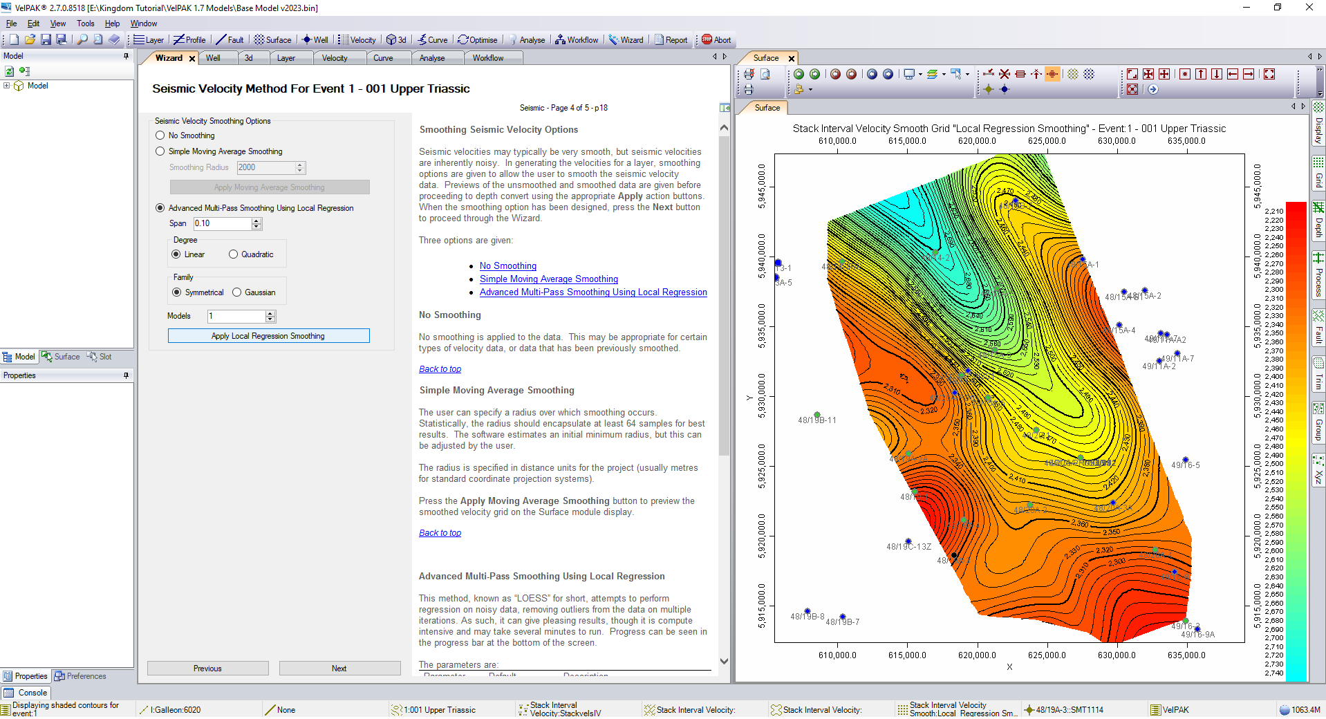
Alternatively, you can choose the Local Regression Smoothing which is more computationally expensive, taking roughly 20 times the length of time to perform the processing, but provides you with a smoother surface to work with. When you have made your selection, press Next.
Click next on this page to complete this step of the sequence.
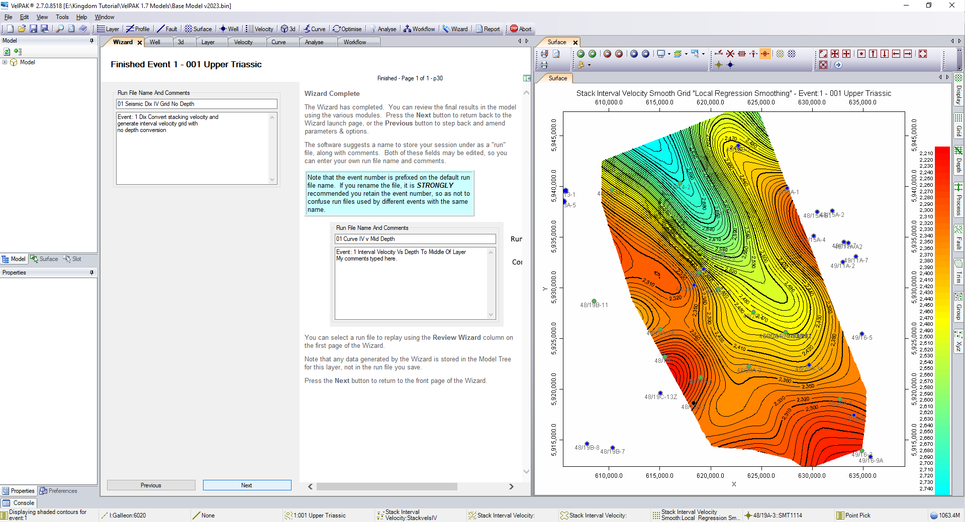
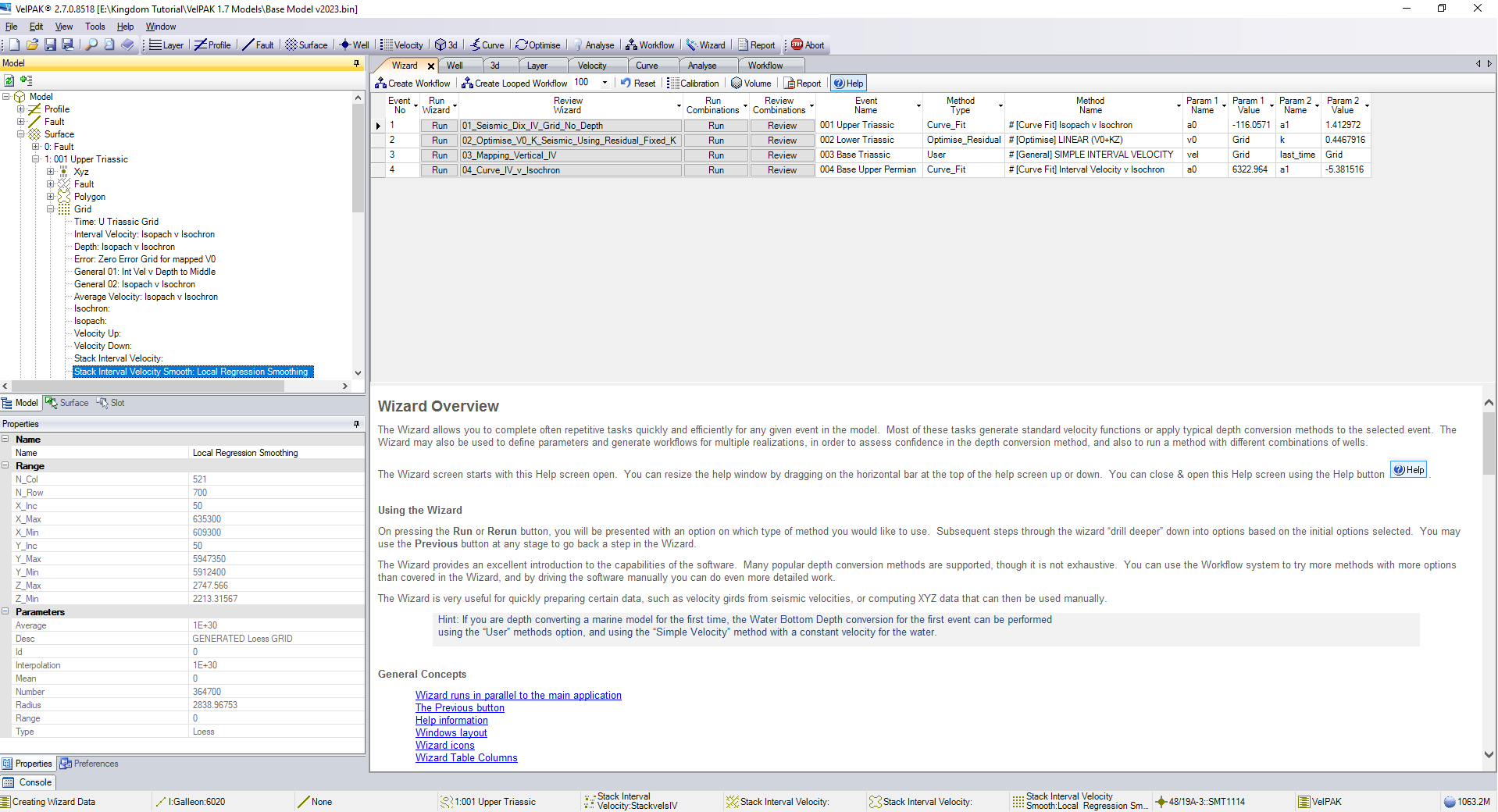
If you close the Surface tab and expend the model tree, you can see that the software has saved the grid you have made in the ‘Stack Interval Velocity Smooth’ slot in the Grid list for the layer you’re working on. To proceed, press Run on Layer 1.
This time around, select the Mapping option and press Next.
The software will check that you have the correct data available and you can press Next to continue.
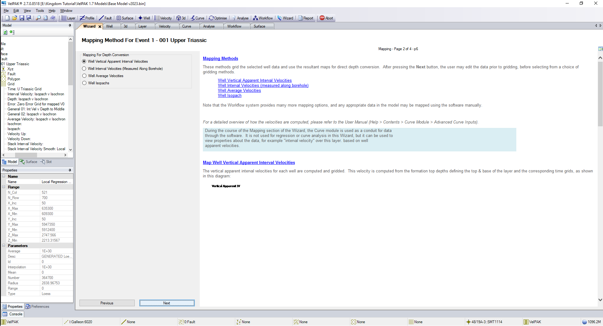
On this page there are several mapping options. In this example you can select the top option to map the Well Vertical Apparent Interval Velocities and then press Next.
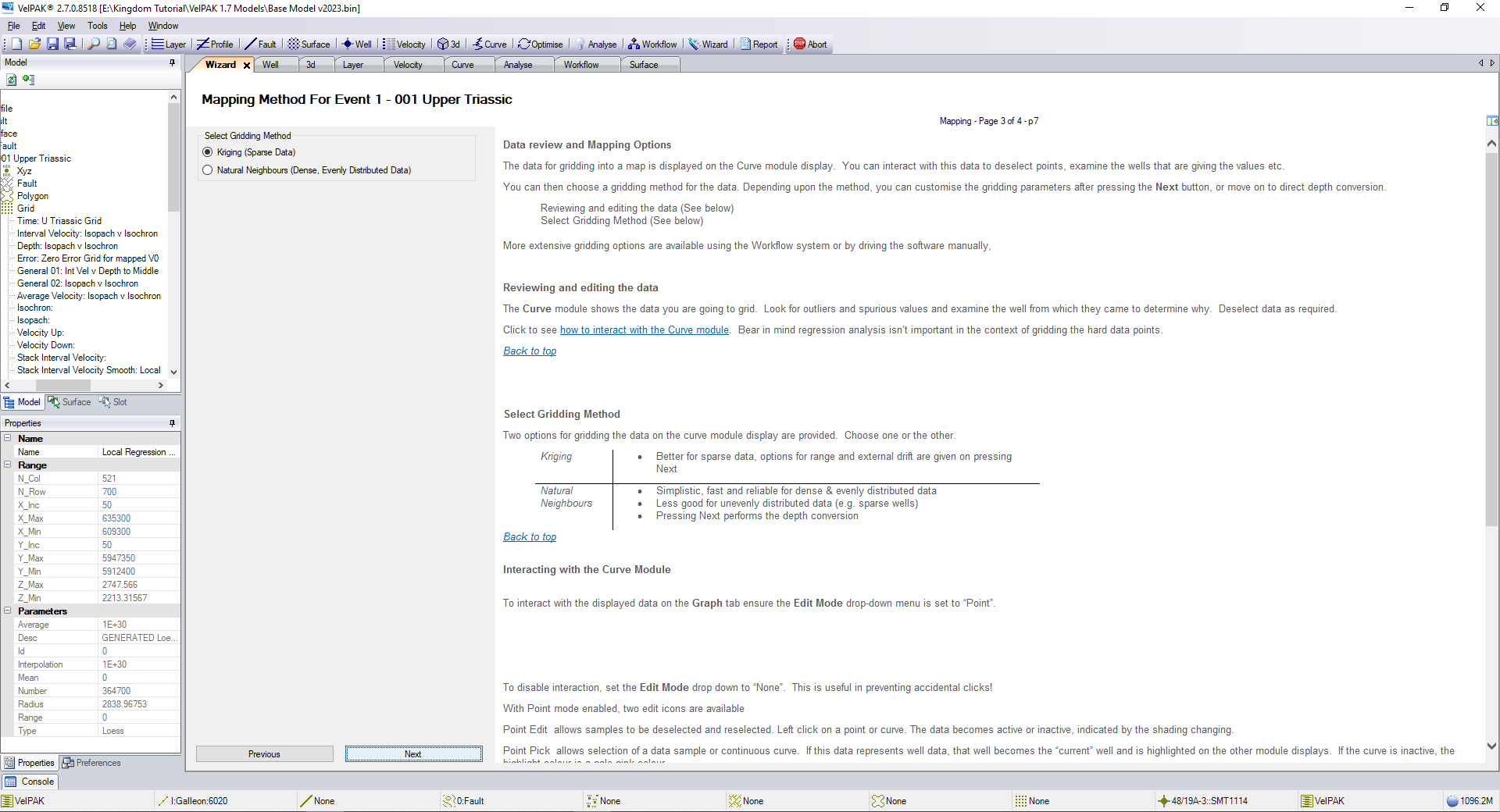
If you have a sparse coverage of wells across your survey area, select the top option to perform kriging. If you have a dense coverage of wells, then you can select the Natural Neighbours option. In this example we’ll proceed with the kriging option and then press Next.
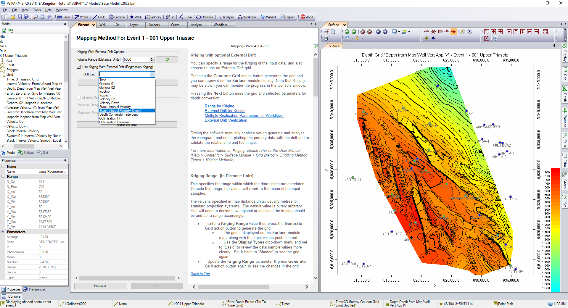
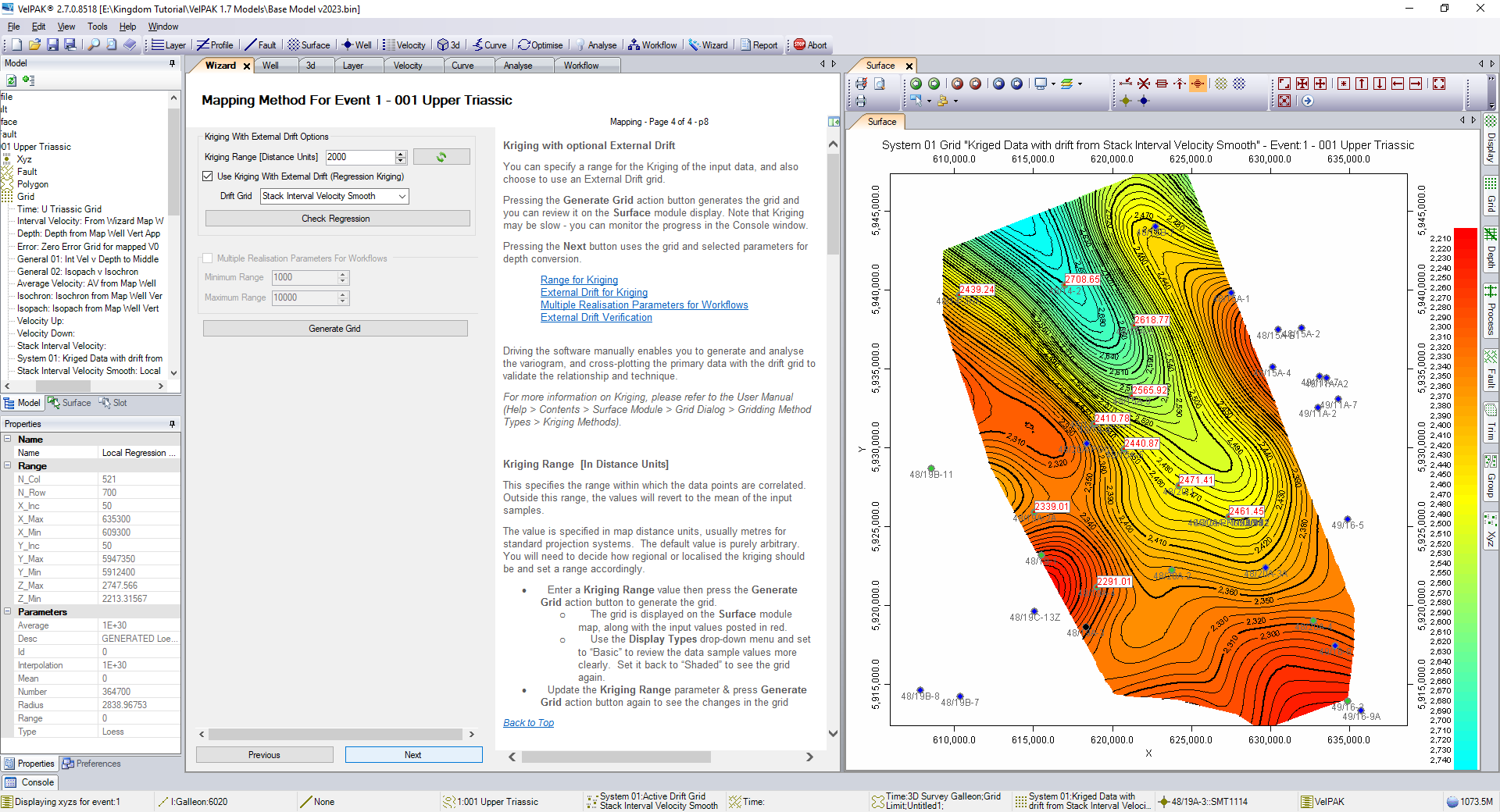
On this page you can select the kriging range. Again this is an arbitrary value which is based on your data. In this example, the value will be changed from 5000 to 2000. You then tick the “Use Kriging With External Drift” box and select the “Stack Interval Velocity Smooth” grid that you generated earlier.
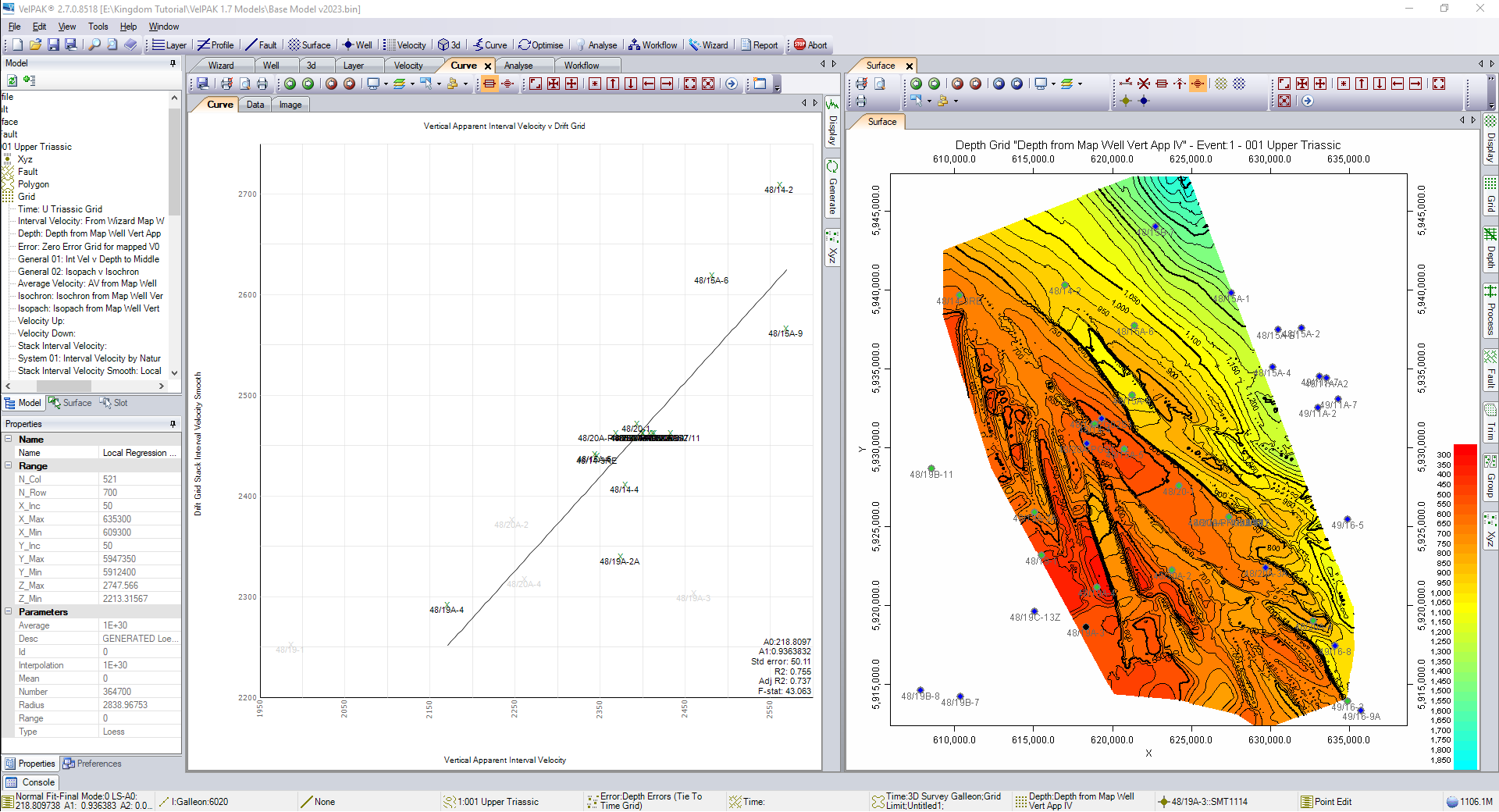
It is important to click on the Check Regression box to evaluate the appropriateness of this technique for your data. You can see in this example (in the bottom right hand corner of the graph) that there is an R2 value of 75.5%. Any correlation over 70% is typically considered viable to work with.
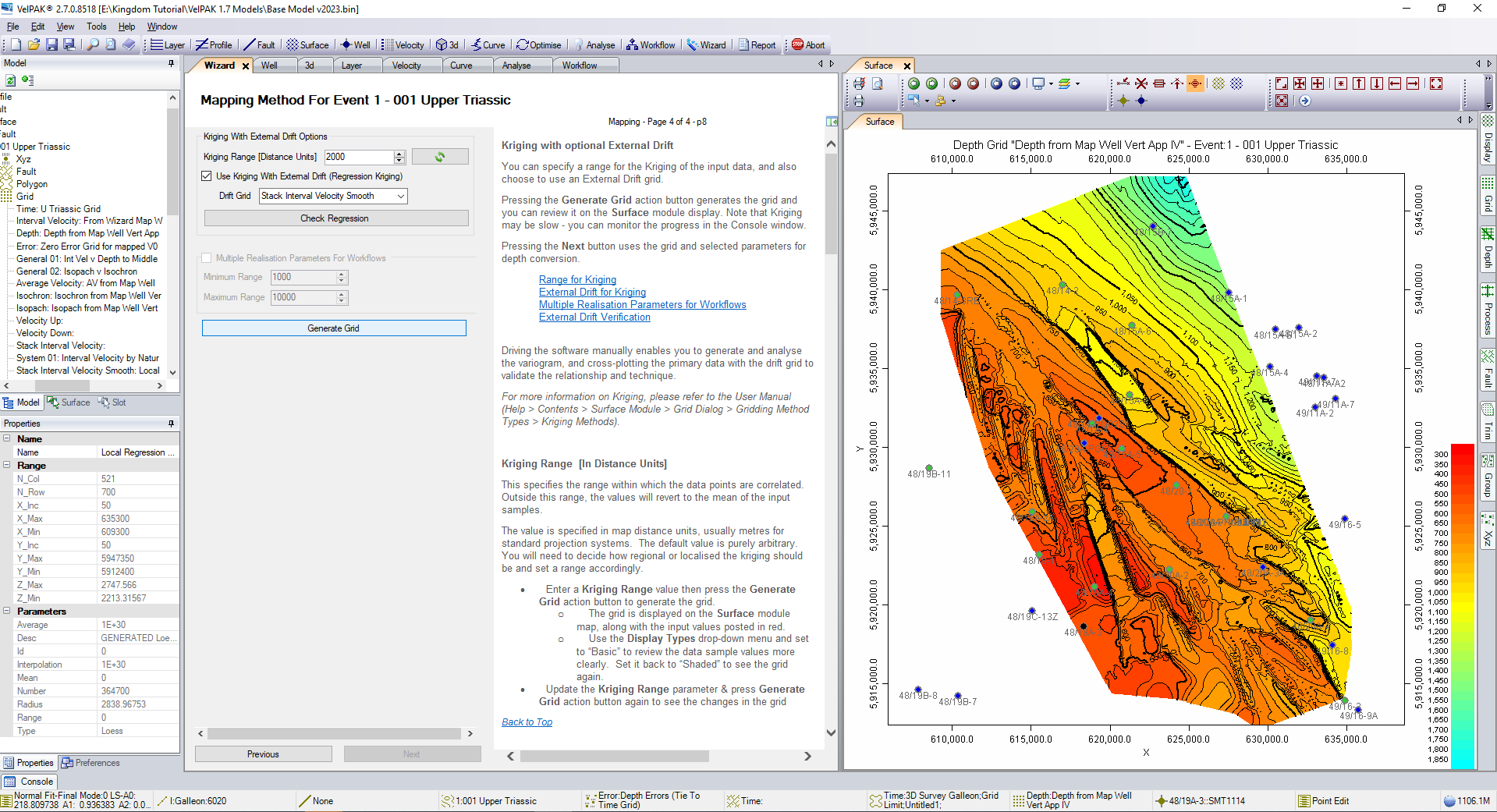
Now click on Generate Grid to process the grid.
As you can see in the example below, the software has computed the Vertical Apparent Interval Velocity values for each of the wells. The external drift grid has been distorted to fit the wells, as defined by your radius, and as you go away from your wells you will default to the soft data of the external grid. This option will provide you with a depth conversion which is significantly more robust than simply contour mapping sparse data.
Press Next 3 times to return to the Wizard.
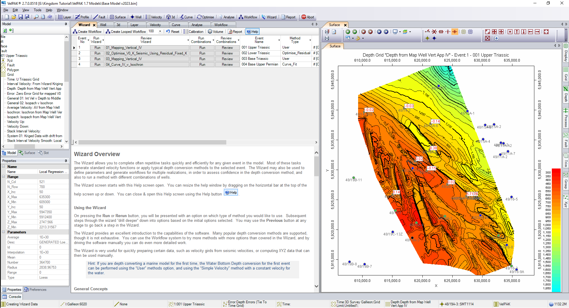
This completes the depth conversion and you will see the map update with the title telling you that you are looking at the Depth Grid “Depth from Map Well Vert App IV” for Event 1. To reiterate the point that the technique is ideal for fairly flat geology with little complexity, but will not necessarily be appropriate to use when the geology becomes progressively more complex.
If you would like to know more about Kingdom’s VelPAK (Velit on Petrel) then click here. Alternatively, you can contact us for a free evaluation by e-mailing us on sales@equipoisesoftware.com.
The software is provided by S&P Global (who we partner with for Kingdom) with perpetual and subscription pricing available on request. We offer a series of Teams meetings throughout the evaluation to help you quickly step up the learning curve and enable you to see the results for yourself.