Upon loading Kingdom Seismic Inversion you are presented with an initial selection screen where you can select the type of Inversion you wish to perform. At this first step, you can select ‘Colored Inversion’ from the menu.
Data Selection Screen
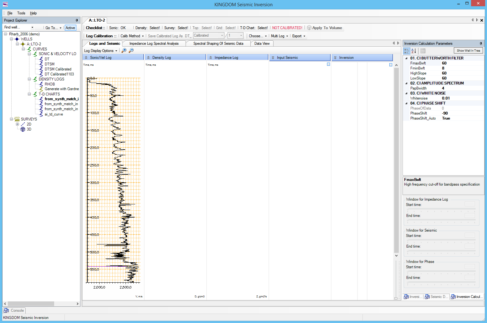
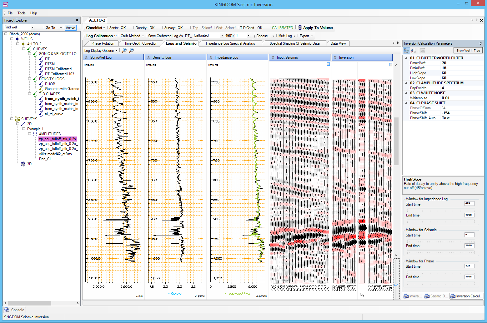
Next is the data selection screen, where you’ll find a model tree to the left-hand-side of the main window. Colored Inversion enables you to perform a multi-well operation by working through each of your wells in turn. In this article we will focus on the steps taken for a single well.
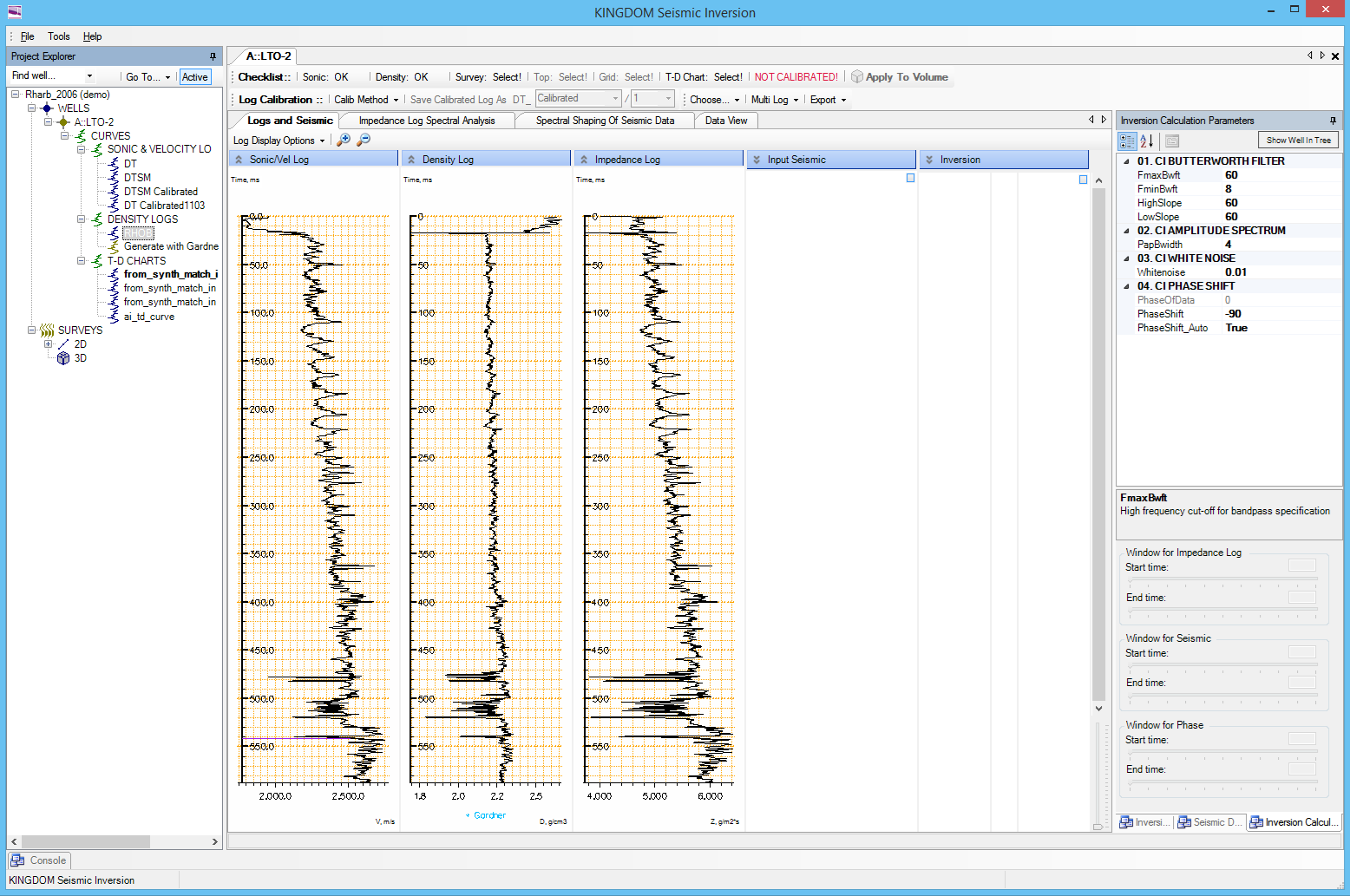
Firstly select your DT, under Curves > Sonic & Velocity Logs. Then select your Density Log and then your Time-Depth chart. You can see that the panel which runs along the top of the screen will change from ‘Select’ to ‘OK’ with each successive click for the respective data types.
Amplitude Volume Selection
Finally select the amplitude volume you wish to work with under Surveys > 2D or 3D > Amplitudes.
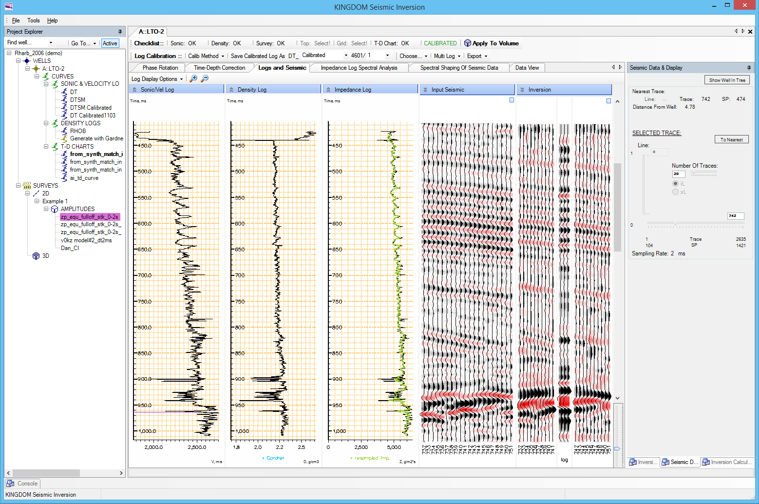
You will see that the main window displays the Sonic/Velocity Log, the Density Log, the Impedance Log, the Input Seismic and the Inversion, the latter showing 3 traces around the well location and 10 traces either side.
Impedance Log Spectral Analysis
Next you can click on the ‘Impedance Log Spectral Analysis’ tab where it displays the Impedance Log in the top left, the Butterworth filter in the top right, the Impedance spectrum in the bottom left and the Modelled spectrum in the bottom right window. This screen is used for QC’ing your data but is not interactive.
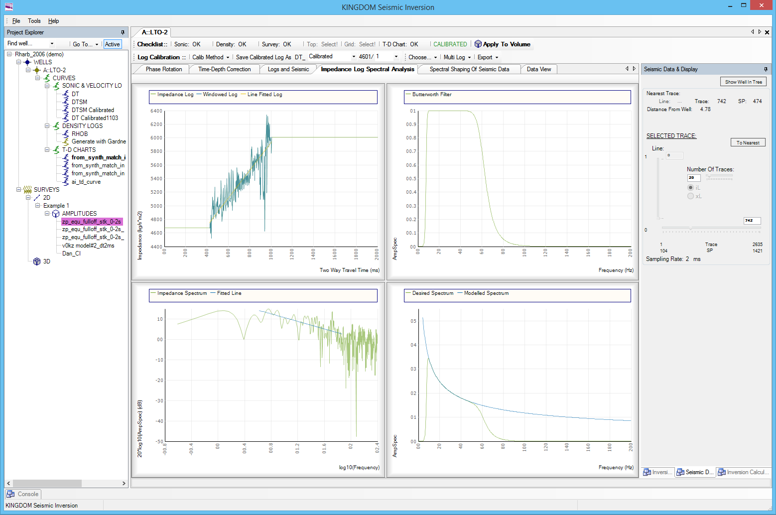
For reflectivity logs, the usual observation is that its amplitude spectrum trend gently rises with frequency – usually described as the “blueness” of the spectrum. The impedance logs however, tend to decay with frequency – having effectively undergone the process of integration relative to the reflectivity data.
The amplitude spectra of the impedance logs (velocity * density) derived for the window of interest can be calculated and displayed on a log-log graph from which a linear spectral slope can be estimated. The fitted line can be expressed as the exponential α in the equivalent representation of the spectral trend in the form A*fα.
Spectral Shaping of Seismic Data
Next you can select the Spectral Shaping of Seismic Data tab.
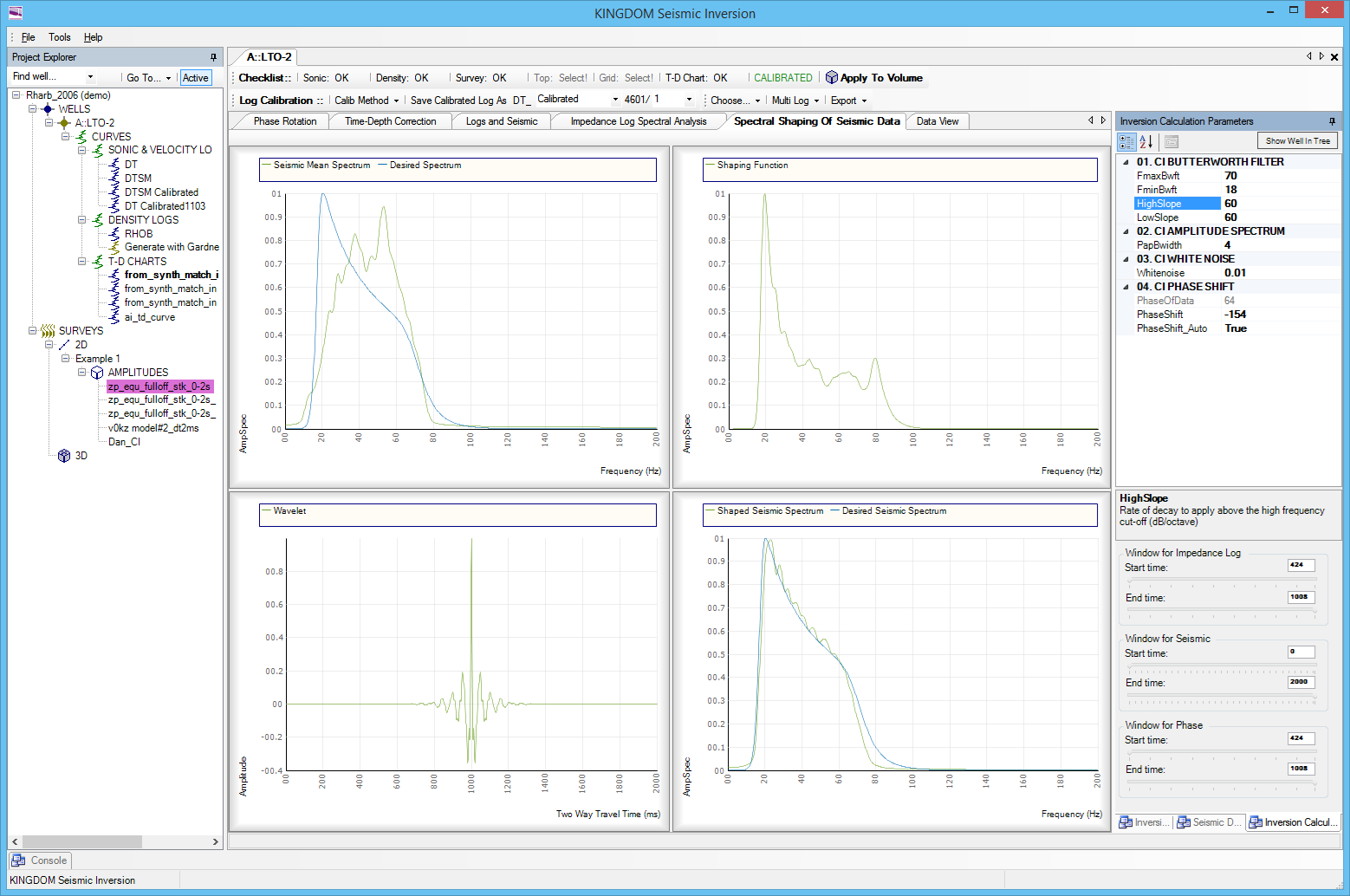
The trend observed in the spectra of the seismic traces must then be matched to the trend of the logs. The seismic spectrum will not in general exhibit the same linear trend behavior, and an operator is therefore computed in the frequency domain to achieve the observed log trend by amplitude multiplication.
A subset of the traces to be input for inversion is selected (and windowed) for spectral analysis as representatives of the complete data set. The amplitude spectra are averaged and smoothed – to enable a smooth spectral shaping operator to be derived to operate on the data.
The smoothing can conveniently be performed within the computation of the amplitude spectrum, by calculating from the autocorrelation of the data. Spectral smoothing is achieved by windowing the autocorrelation – a Papoulis window enables this to be done in a controlled manner without introducing undesirable side-lobes in the spectrum.
Top Left: Average seismic spectrum superimposed by the desired impedance log spectrum
Top Right: A derived operator in the frequency domain
Bottom Left: A derived operator in the time domain
Bottom right: Shaped seismic spectrum superimposed by the desired impedance log spectrum
Here you can adjust the parameters applied to the Butterworth Filter by selecting the Inversion Calculation Parameters tab at the bottom left of the side panel. In this instance I have selected the FmaxBwft to be 70 and the FminBwft to be 18 to optimally derive the desired seismic spectrum.
Phase Rotation
Once you are happy with your selection parameters, you can move onto the Phase Rotation tab.
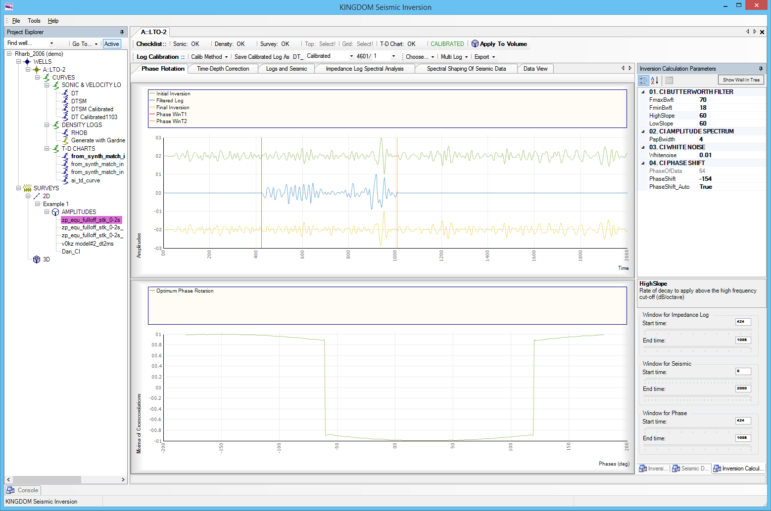
When the input seismic traces have been accurately zero-phased relative to the reflectivity sequence at wells, the coloured inversion process requires a phase shift of -90° to complete the match with the impedance log as well as the estimated amplitude spectral trend.
Many data sets as delivered for interpretation have been zero-phased (or zero-phasing has at least been attempted). However, frequently the phase of the data is unknown, or the zero-phasing has been inaccurate, and in many cases the polarity of the seismic is unknown or ambiguously defined.
There is an opportunity in the inversion package to apply a phase shift that will optimise the tie with impedance log traces, or the program can be requested to calculate the phase. The program estimates the phase rotation angle by comparing bandpass filtered impedance logs with the shaped seismic data assuming that well ties are reasonably good.
This phase value will be used to rotate the shaped seismic data to complete the coloured inversion process.
Top: Shaped seismic trace (green), filtered impedance log (blue) and phase rotated seismic trace (inversion result)
Bottom: Cost-function for angles between -180º and 180º
Logs and Seismic
Next, we can move onto the Logs and Seismic screen.
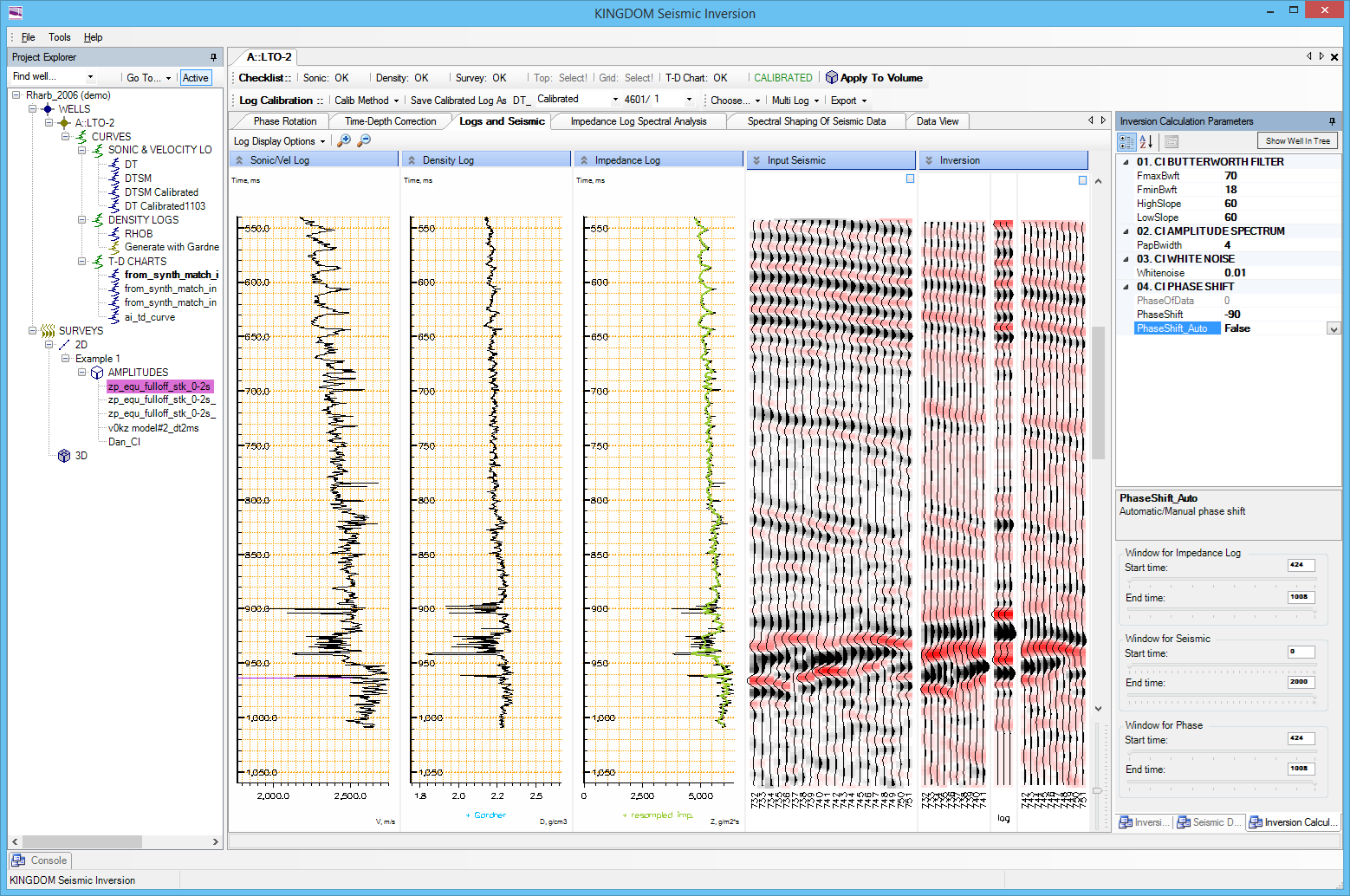
A unique feature of our Coloured Inversion software is the automatic phase shift algorithm. Here we can see the inversion with the phase shift off (false).
Here we can see the phase shift on (True). By comparing these two images, it can be seen that the automatic phase shift enhances the quality of the inversion, where the inversion has less noise and less signal instability and aligns more closely with the well traces.
Apply to Volume
When you are satisfied with the inversion parameters you have selected, the last step is to select ‘Apply To Volume’ at the top of the screen.
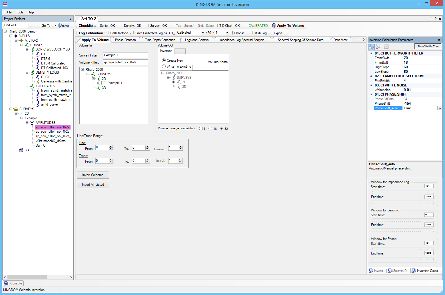
On this screen we write a relative impedance volume as a new file, or to overwrite an existing file.
A Coloured Inversion operator can be derived from either single well or multiple wells. The inversion process is a simple application of a filter operator to the input seismic data followed by a phase rotation of shaped traces.
For a 3D seismic volume, you can select inline and cross line ranges to invert.
You can adjust the Line/Trace Range and then press the Invert Selected button to start the inversion running. It is very fast to invert a whole volume, with operations under an hour, even for very large datasets.
The results can be viewed immediately by selecting the data back in the Kingdom software. There is a nuance to the software that you need to completely close Kingdom and reopen it again for the data to become visible.
This concludes the entire process of operating Kingdom’s Colored Inversion module. You’ll note that once you’ve selected your data, you only really have to interact with the 4 parameters of the Butterworth filter to get your Shaped Seismic Spectrum to match your Desired Seismic Spectrum and then click on Invert! Hopefully you can see how easy this operation is to do and how it can maximise the value of your seismic data, making it easier to perform your interpretation on, as you can see in these two final images:
Colored Inversion Example
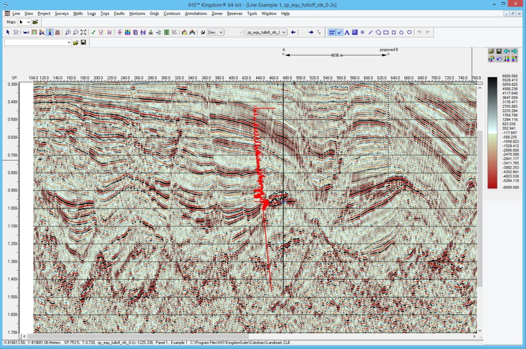
Original Seismic Section
Colored Inversion Display
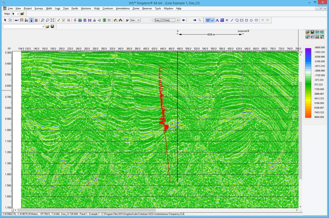
You can see that in the Colored Inverted section that the low impedance values are highlighted in dark blue and stand out from the surrounding geology, maximising the value of your seismic data. “Colored Inversion is the ideal point at which to begin any Seismic Interpretation”.
If you’d like to know more about Kingdom Seismic Inversion then click here or to contact us for a free evaluation e-mail us on sales@equipoisesoftware.com.
The software is provided by S&P Global (who we partner with for Kingdom) with perpetual and subscription pricing available on request. We offer a series of Teams meetings throughout the evaluation to help you quickly step up the learning curve and enable you to see the results for yourself.