In this month’s behind the scenes look at LogToVolume, which is coming soon to provide you with next generation depth conversion, we explore the Depth Conversion element of the toolset.
The following snapshots of the software are not in a finished state, as they are missing icons and the final aesthetic details of the finished product. However, you will get a feel for the ease-of-use of the tool and gain an understanding of the step-by-step nature of the final result.
Following on from the LogSpread article which we covered last month, and once we have the model created using the LogSpread tool, the next step of the process is to then depth convert that volume.
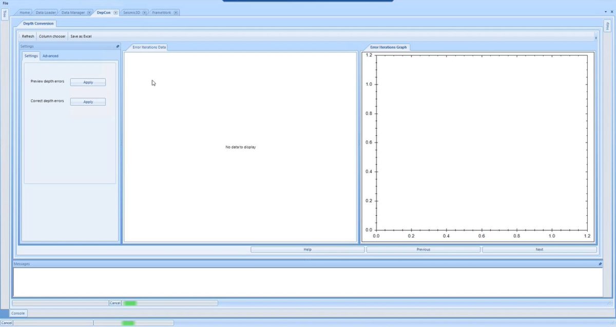
As you can see in the image below, the software provides you with the ability to preview the depth errors or just move through to Correct the depth errors.
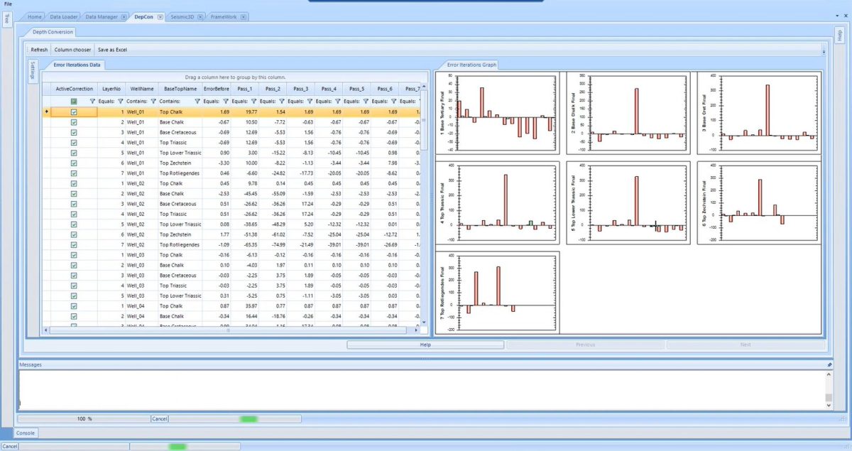
Upon selecting Preview depth errors, you are presented with this screen which gives you an overview of the steps taken by the software to come to its final result. The software works by completing a series of ‘passes’ by iteratively improving the results from layer to layer. In this example, we have a 7-layer depth model, and so the software performs a pass per layer, per well. The error iterations graphs then display the residual values for each well per layer. If you look at these graphs, it is immediately obvious that Well_07 has large discrepancies with the error being represented as the tall bar on the plots. In this case, the preference would be for you to go back to Kingdom and correct the data and start from this point again. Alternatively, you can simply untick Well_07 from the wells in the Active Correction column to turn it off from the calculations.
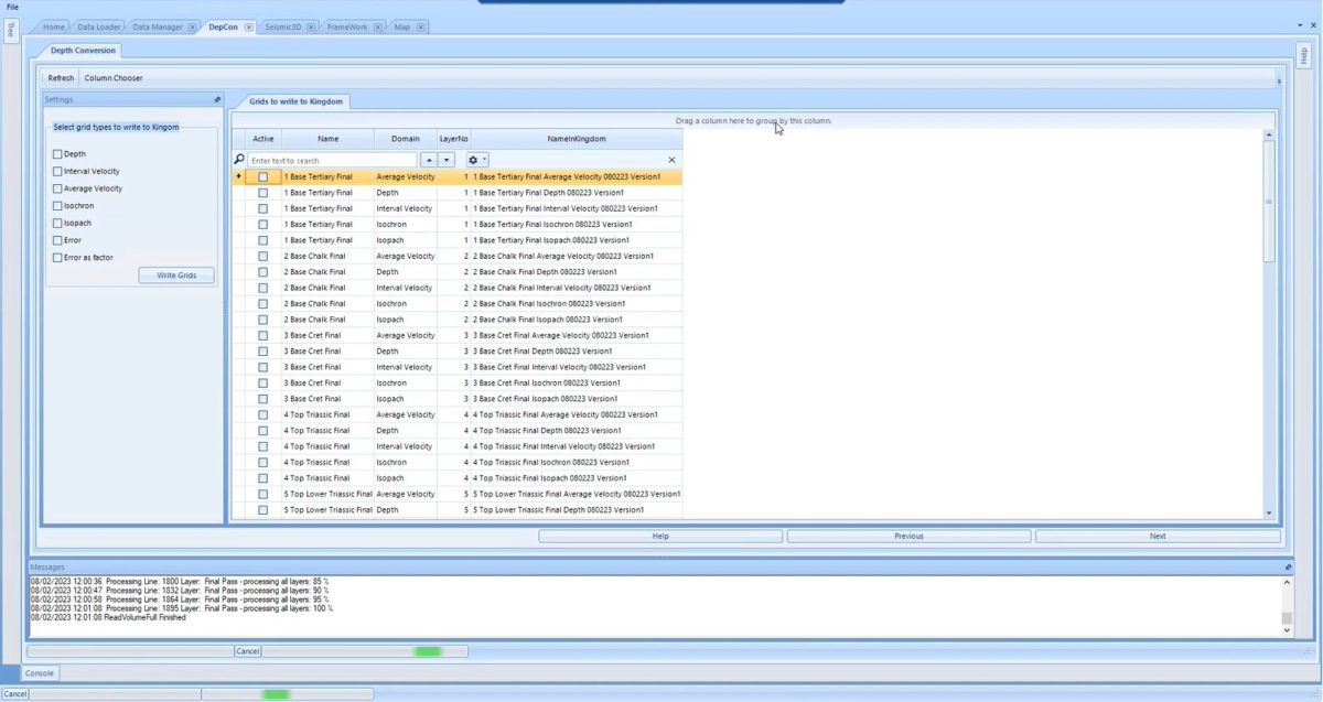
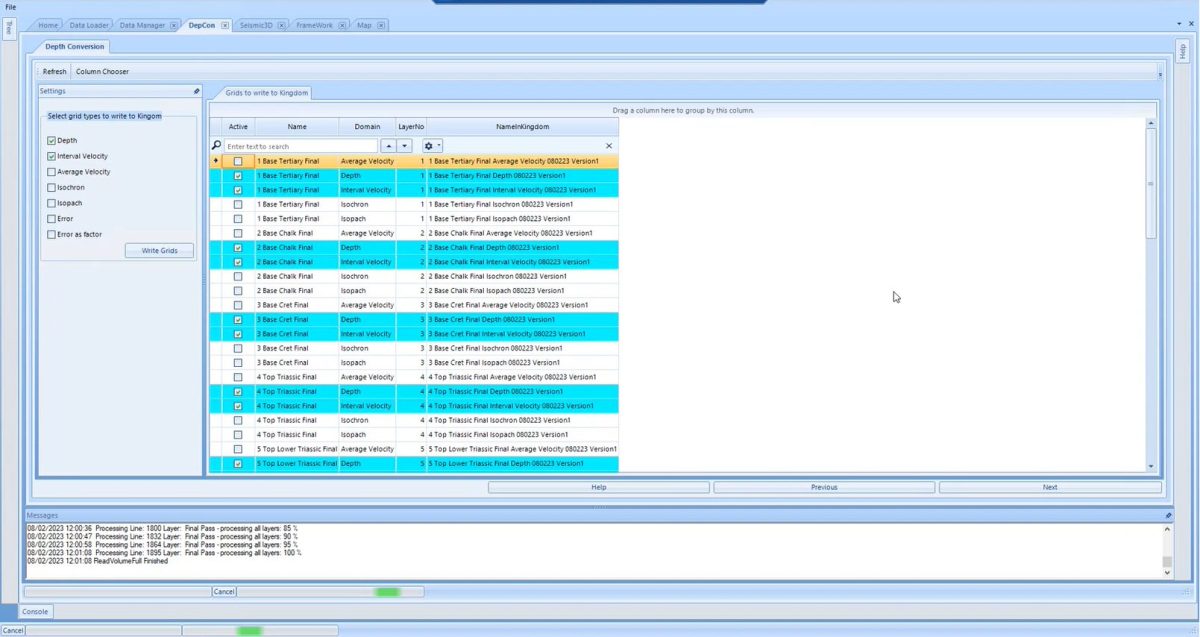
When you are happy with the data that you’ve selected to work with in the model, you’ll then get the software to perform the ‘passes’ in full and this processing can take several minutes to compute. Once these grids have been processed, you have the option to output any of the grids that you’ve made to Kingdom. These can be Depth, Interval Velocity, Average Velocity, Isochron, Isopach, Error or Error as a factor. This is a tick box exercise and you can select as much or little data as you want to transfer and can use the grouping option so that, for example, all your depth grids can be brought across in one click.
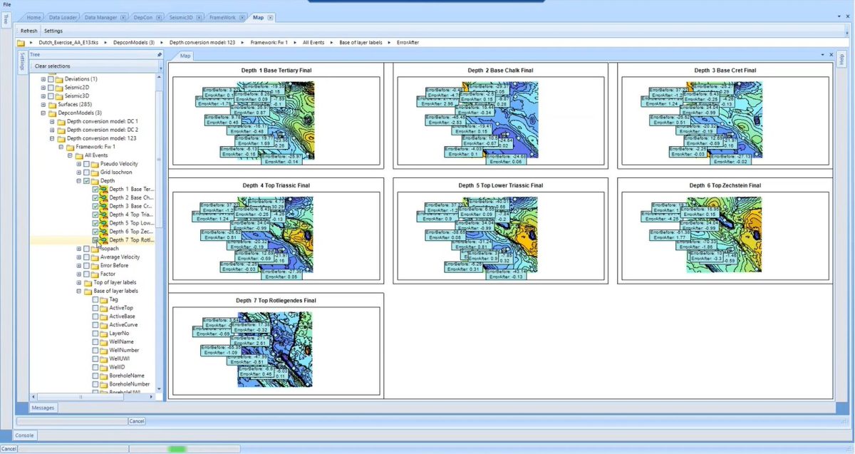
The software also permits you to view any of the data you have created, as well as post information on the maps for each of the layers. Each of the maps are linked, so that as you zoom in on one of them, all of the other maps will zoom in simultaneously. You can also untick any maps you don’t want to view, or opt to view a single map within the window. This is all selected in the model tree and uses a tick box operation to select the visible layers and the data you want to display.
When you’ve completed your selection you can click the Write Grids button and the relevant data will be synchronised with Kingdom. The program is tightly linked with Kingdom such that the data is then immediately visible in the Kingdom tree. Due to the sheer number of grids that could be output, it can be recommended to make a new folder in Kingdom’s model tree and copy the LogToVolume grids into that location, for good house keeping of your data.
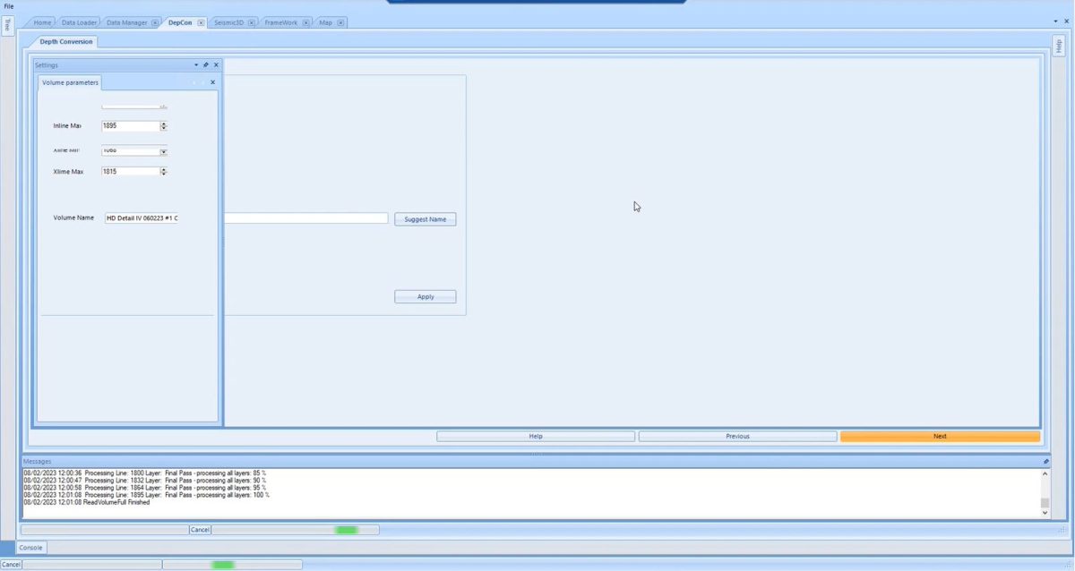
The next step in the process is the final volume creation. On this page, you can select the InLine and XLine ranges and select a name for the volume, or click Suggest Name to have the software populate that box for you.
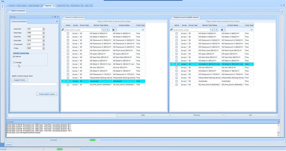
You are then presented with the option to create an Interval or Average velocity volume and can select the relevant data from the lists. The first column of data is asking you to select the volume you wish to convert, in this case the Seismic Amplitude volume. The second column of data is asking for the velocity volume you want to use to perform the conversion. In this case, we’ve selected the corrected volume that we’ve created on the journey to get to this page. You then press ‘Create depth Volume’ and let the software complete the process, which would take roughly an hour.
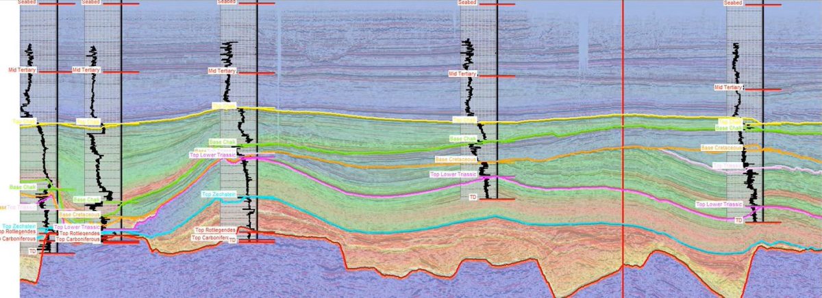
When this volume has been processed, you will then be able to access it in Kingdom as the seismic volume in the depth domain. In the image below you can see that we’ve used the overlay to display the velocity volume over the seismic, which is a robust depth conversion which ties the wells at all locations. You can also see that the velocities within the layers encompass the geological complexity of the data, thus ensuring a very reliable result.
You can hopefully see how you will be able to generate quite powerful and useful products in this very easy to use Wizard.
If you have any questions about the new developments of our software, or want to discuss our other products, or the depth conversion training courses we provide, then please get in touch with us at sales@equipoisesoftware.com where we’ll be happy to discuss your questions in more detail.